Principal Components Analysis

Perform a principal components analysis (PCA) on a matrix or data frame and return a pcomp object.

Usage

pcomp(x, ...)

# S3 method for formula
pcomp(formula, data = NULL, subset, na.action, method = c("svd", "eigen"), ...)

# S3 method for default
pcomp(
  x,
  method = c("svd", "eigen"),
  scores = TRUE,
  center = TRUE,
  scale = TRUE,
  tol = NULL,
  covmat = NULL,
  subset = rep(TRUE, nrow(as.matrix(x))),
  ...
)

# S3 method for pcomp
print(x, ...)

# S3 method for pcomp
summary(object, loadings = TRUE, cutoff = 0.1, ...)

# S3 method for summary.pcomp
print(x, digits = 3, loadings = x$print.loadings, cutoff = x$cutoff, ...)

# S3 method for pcomp
plot(
  x,
  which = c("screeplot", "loadings", "correlations", "scores"),
  choices = 1L:2L,
  col = par("col"),
  bar.col = "gray",
  circle.col = "gray",
  ar.length = 0.1,
  pos = NULL,
  labels = NULL,
  cex = par("cex"),
  main = paste(deparse(substitute(x)), which, sep = " - "),
  xlab,
  ylab,
  ...
)

# S3 method for pcomp
screeplot(
  x,
  npcs = min(10, length(x$sdev)),
  type = c("barplot", "lines"),
  col = "cornsilk",
  main = deparse(substitute(x)),
  ...
)

# S3 method for pcomp
points(
  x,
  choices = 1L:2L,
  type = "p",
  pch = par("pch"),
  col = par("col"),
  bg = par("bg"),
  cex = par("cex"),
  ...
)

# S3 method for pcomp
lines(
  x,
  choices = 1L:2L,
  groups,
  type = c("p", "e"),
  col = par("col"),
  border = par("fg"),
  level = 0.9,
  ...
)

# S3 method for pcomp
text(
  x,
  choices = 1L:2L,
  labels = NULL,
  col = par("col"),
  cex = par("cex"),
  pos = NULL,
  ...
)

# S3 method for pcomp
biplot(x, choices = 1L:2L, scale = 1, pc.biplot = FALSE, ...)

# S3 method for pcomp
pairs(
  x,
  choices = 1L:3L,
  type = c("loadings", "correlations"),
  col = par("col"),
  circle.col = "gray",
  ar.col = par("col"),
  ar.length = 0.05,
  pos = NULL,
  ar.cex = par("cex"),
  cex = par("cex"),
  ...
)

# S3 method for pcomp
predict(object, newdata, dim = length(object$sdev), ...)

# S3 method for pcomp
correlation(x, newvars, dim = length(x$sdev), ...)

scores(x, ...)

# S3 method for pcomp
scores(x, labels = NULL, dim = length(x$sdev), ...)

Arguments

x: A matrix or data frame with numeric data.
...: Arguments passed to or from other methods. If x is a formula one might specify scale, tol or covmat.
formula: A formula with no response variable, referring only to numeric variables.
data: An optional data frame (or similar, see model.frame()) containing the variables in the formula. By default the variables are taken from environment(formula).
subset: An optional vector used to select rows (observations) of the data matrix x.
na.action: A function which indicates what should happen when the data contain NAs. The default is set by the na.action setting of options(), and is na.fail() if that is not set. The 'factory-fresh' default is na.omit().
method: Either "svd" (using prcomp()), "eigen" (using princomp()), or an abbreviation.
scores: A logical value indicating whether the score on each principal component should be calculated.
center: A logical value indicating whether the variables should centered. Alternately, a vector of length equal the number of columns of x can be supplied. The value is passed to scale. Note that this argument is ignored for method = "eigen" and the dataset is always centered in this case.
scale: A logical value indicating whether the variables should be scaled to have unit variance before the analysis takes place. The default is TRUE, which in general, is advisable. Alternatively, a vector of length equal the number of columns of x can be supplied. The value is passed to scale().
tol: Only when method = "svd". A value indicating the magnitude below which components should be omitted. (Components are omitted if their standard deviations are less than or equal to tol times the standard deviation of the first component.) With the default null setting, no components are omitted. Other settings for tol = could be tol = 0 or tol = sqrt(.Machine$double.eps), which would omit essentially constant components.
covmat: A covariance matrix, or a covariance list as returned by cov.wt() (and cov.mve() or cov.mcd() from package MASS). If supplied, this is used rather than the covariance matrix of x.
object: A 'pcomp' object.
loadings: Do we also summarize the loadings?
cutoff: The cutoff value below which loadings are replaced by white spaces in the table. That way, larger values are easier to spot and to read in large tables.
digits: The number of digits to print.
which: The graph to plot.
choices: Which principal axes to plot. For 2D graphs, specify two integers.
col: The color to use in graphs.
bar.col: The color of bars in the screeplot.
circle.col: The color for the circle in the loadings or correlations plots.
ar.length: The length of the arrows in the loadings and correlations plots.
pos: The position of text relative to arrows in loadings and correlation plots.
labels: The labels to write. If NULL default values are computed.
cex: The factor of expansion for text (labels) in the graphs.
main: The title of the graph.
xlab: The label of the x-axis.
ylab: The label of the y-axis.
npcs: The number of principal components to represent in the screeplot.
type: The type of screeplot ("barplot" or "lines") or pairs plot ("loadings" or "correlations").
pch: The type of symbol to use.
bg: The background color for symbols.
groups: A grouping factor.
border: The color of the border.
level: The probability level to use to draw the ellipse.
pc.biplot: Do we create a Gabriel's biplot (see biplot())?
ar.col: Color of arrows.
ar.cex: Expansion factor for text on arrows.
newdata: New individuals with observations for the same variables as those used for calculating the PCA. You can then plot these additional individuals in the scores plot.
dim: The number of principal components to keep.
newvars: New variables with observations for same individuals as those used for calculating the PCA. Correlation with PCs is calculated. You can then plot these additional variables in the correlation plot.

Value

A c("pcomp", "pca", "princomp") object.

Details

pcomp() is a generic function with "formula" and "default" methods. It is essentially a wrapper around prcomp() and princomp() to provide a coherent interface and object for both methods.

A 'pcomp' object is created. It inherits from 'pca' (as in labdsv package, but not compatible with the version of 'pca' in ade4) and of 'princomp'.

For more information on algorithms, refer to prcomp() for method = "svd" or princomp() for method = "eigen".

Note

The signs of the columns for the loadings and scores are arbitrary. So, they could differ between functions for PCA, and even between different builds of R.

Author

Philippe Grosjean phgrosjean@sciviews.org, but the core code is indeed in package stats.

Examples

# Let's analyze mtcars without the Mercedes data (rows 8:14)
data(mtcars)
cars.pca <- pcomp(~ mpg + cyl + disp + hp + drat + wt + qsec,
  data = mtcars, subset = -(8:14))
cars.pca
#> Call:
#> pcomp(formula = ~mpg + cyl + disp + hp + drat + wt + qsec, data = mtcars, 
#>     subset = -(8:14))
#> 
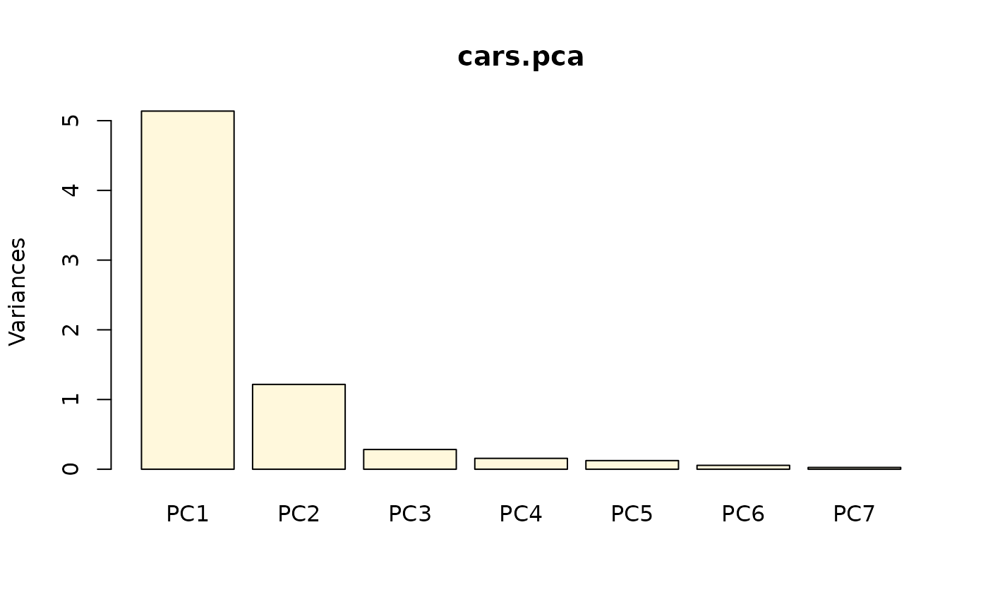
#> Variances:
#>        PC1        PC2        PC3        PC4        PC5        PC6        PC7 
#> 5.13759552 1.21698212 0.28325478 0.15620899 0.12409321 0.05604916 0.02581622 
#> 
#>  7  variables and  25 observations.
summary(cars.pca)
#> Importance of components (eigenvalues):
#>                          PC1   PC2    PC3    PC4    PC5     PC6     PC7
#> Variance               5.138 1.217 0.2833 0.1562 0.1241 0.05605 0.02582
#> Proportion of Variance 0.734 0.174 0.0405 0.0223 0.0177 0.00801 0.00369
#> Cumulative Proportion  0.734 0.908 0.9483 0.9706 0.9883 0.99631 1.00000
#> 
#> Loadings (eigenvectors, rotation matrix):
#>      PC1    PC2    PC3    PC4    PC5    PC6    PC7   
#> mpg  -0.415         0.107 -0.754 -0.353 -0.318  0.144
#> cyl   0.425         0.165 -0.447  0.289  0.485  0.521
#> disp  0.423  0.110 -0.234 -0.465  0.103        -0.726
#> hp    0.385 -0.349 -0.106        -0.817  0.203       
#> drat -0.320 -0.505 -0.736         0.208  0.222       
#> wt    0.400  0.262 -0.499               -0.590  0.416
#> qsec -0.240  0.733 -0.323        -0.267  0.475       
screeplot(cars.pca)


# Loadings are extracted and plotted this way:
(cars.ldg <- loadings(cars.pca))
#> 
#> Loadings:
#>      PC1    PC2    PC3    PC4    PC5    PC6    PC7   
#> mpg  -0.415         0.107 -0.754 -0.353 -0.318  0.144
#> cyl   0.425         0.165 -0.447  0.289  0.485  0.521
#> disp  0.423  0.110 -0.234 -0.465  0.103        -0.726
#> hp    0.385 -0.349 -0.106        -0.817  0.203       
#> drat -0.320 -0.505 -0.736         0.208  0.222       
#> wt    0.400  0.262 -0.499               -0.590  0.416
#> qsec -0.240  0.733 -0.323        -0.267  0.475       
#> 
#>                  PC1   PC2   PC3   PC4   PC5   PC6   PC7
#> SS loadings    1.000 1.000 1.000 1.000 1.000 1.000 1.000
#> Proportion Var 0.143 0.143 0.143 0.143 0.143 0.143 0.143
#> Cumulative Var 0.143 0.286 0.429 0.571 0.714 0.857 1.000
plot(cars.pca, which = "loadings") # Equivalent to vectorplot(cars.ldg)


# Similarly, correlations of variables with PCs are extracted and plotted:
(cars.cor <- Correlation(cars.pca))
#> Matrix of PCA variables and components correlation:
#>      PC1    PC2    PC3    PC4    PC5    PC6    PC7   
#> mpg  -0.940 -0.055  0.057 -0.298 -0.124 -0.075  0.023
#> cyl   0.963 -0.062  0.088 -0.177  0.102  0.115  0.084
#> disp  0.960  0.122 -0.124 -0.184  0.036  0.003 -0.117
#> hp    0.873 -0.385 -0.056  0.039 -0.288  0.048  0.005
#> drat -0.726 -0.557 -0.392 -0.030  0.073  0.053  0.009
#> wt    0.906  0.289 -0.266  0.006  0.004 -0.140  0.067
#> qsec -0.544  0.808 -0.172 -0.010 -0.094  0.112  0.010
plot(cars.pca, which = "correlations") # Equivalent to vectorplot(cars.cor)
# One can add supplementary variables on this graph
lines(Correlation(cars.pca,
  newvars = mtcars[-(8:14), c("vs", "am", "gear", "carb")]))


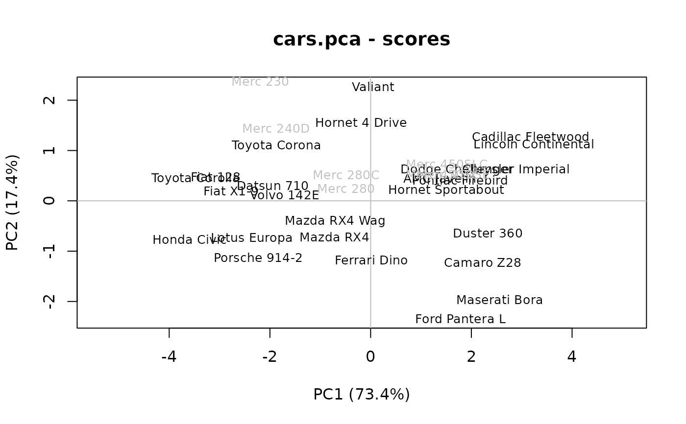
# Plot the scores:
plot(cars.pca, which = "scores", cex = 0.8) # Similar to plot(scores(x)[, 1:2])
#> Warning: NAs introduced by coercion
# Add supplementary individuals to this plot (labels), also points() or lines()
text(predict(cars.pca, newdata = mtcars[8:14, ]),
  labels = rownames(mtcars[8:14, ]), col = "gray", cex = 0.8)


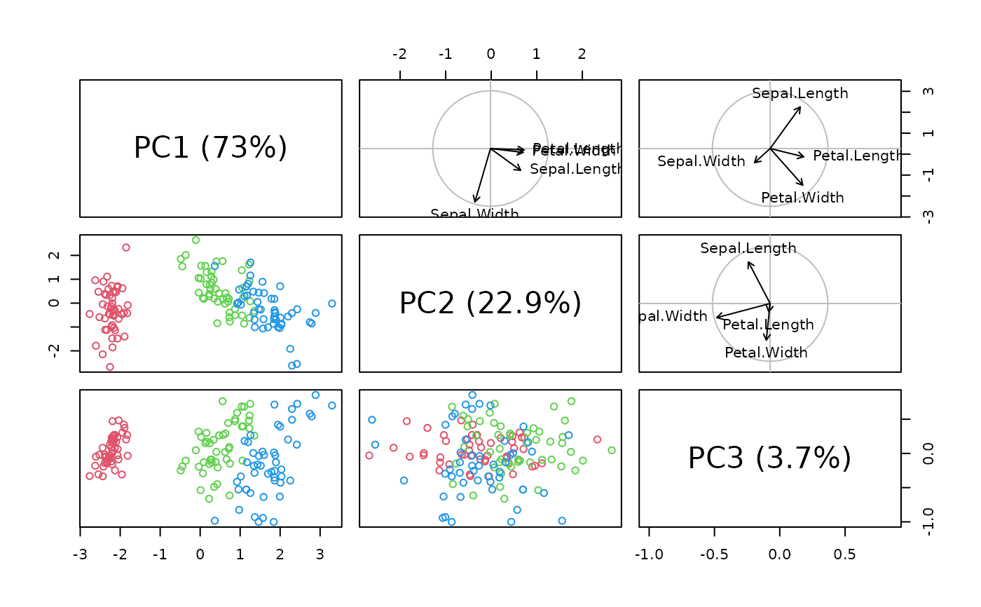
# Pairs plot for 3 PCs
iris.pca <- pcomp(iris[, -5])
pairs(iris.pca, col = (2:4)[iris$Species])