Correspondence Analysis (CA) — ca • exploreit

ca() is a reexport of the function from the ca package, it offers a ca(formula, data, ...) interface. It is supplemented here with various chart() types.

ca(obj, ...)

# S3 method for ca
autoplot(
  object,
  choices = 1L:2L,
  type = c("screeplot", "altscreeplot", "biplot"),
  col = "black",
  fill = "gray",
  aspect.ratio = 1,
  repel = FALSE,
  ...
)

# S3 method for ca
chart(
  data,
  choices = 1L:2L,
  ...,
  type = c("screeplot", "altscreeplot", "biplot"),
  env = parent.frame()
)

Arguments

obj: A formula or a data frame with numeric columns, or a matrix, or a table or xtabs two-way contingency table, see ca::ca(). The formula version allows to specify two categorical variables from a data frame as ~f1 + f2. The other versions analyze a two-way contingency table crossing two factors.
...: Further arguments from ca::ca() or for plot.
object: A pcomp object
choices: Vector of two positive integers. The two axes to plot, by
type: The type of plot to produce: "screeplot" or "altscreeplot" for two versions of the screeplot, or "biplot" for the CA biplot.
col: The color for the points representing the observations, black by default.
fill: The color to fill bars, gray by default
aspect.ratio: height/width of the plot, 1 by default (for plots where the ratio height / width does matter)
repel: Logical. Should repel be used to rearrange points labels? FALSEby default
data: Idem
env: The environment where to evaluate code, parent.frame() by default, which should not be changed unless you really know what you are doing!

Value

pca() produces a ca object.

Examples

library(chart)
data(caith, package = "MASS")
caith # A two-way contingency table
#>        fair red medium dark black
#> blue    326  38    241  110     3
#> light   688 116    584  188     4
#> medium  343  84    909  412    26
#> dark     98  48    403  681    85
class(caith) # in a data frame
#> [1] "data.frame"
caith_ca <- ca(caith)
summary(caith_ca)
#> 
#> Principal inertias (eigenvalues):
#> 
#>  dim    value      %   cum%   scree plot               
#>  1      0.199245  86.6  86.6  **********************   
#>  2      0.030087  13.1  99.6  ***                      
#>  3      0.000859   0.4 100.0                           
#>         -------- -----                                 
#>  Total: 0.230191 100.0                                 
#> 
#> 
#> Rows:
#>     name   mass  qlt  inr    k=1 cor ctr    k=2 cor ctr  
#> 1 | blue |  133  979  111 |  400 836 107 |  165 143 121 |
#> 2 | lght |  293  995  259 |  441 956 286 |   88  39  76 |
#> 3 | medm |  329  999   88 |  -34  18   2 | -245 981 657 |
#> 4 | dark |  244 1000  543 | -703 965 605 |  134  35 145 |
#> 
#> Columns:
#>     name   mass  qlt  inr     k=1 cor ctr    k=2 cor ctr  
#> 1 | fair |  270 1000  383 |   544 907 401 |  174  93 271 |
#> 2 |  red |   53  803   16 |   233 770  14 |   48  33   4 |
#> 3 | medm |  397 1000   78 |    42  39   4 | -208 961 572 |
#> 4 | dark |  258 1000  401 |  -589 969 449 |  104  30  93 |
#> 5 | blck |   22  998  122 | -1094 934 132 |  286  64  60 |

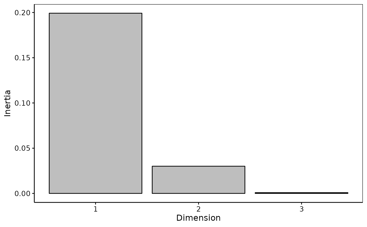
chart$scree(caith_ca)

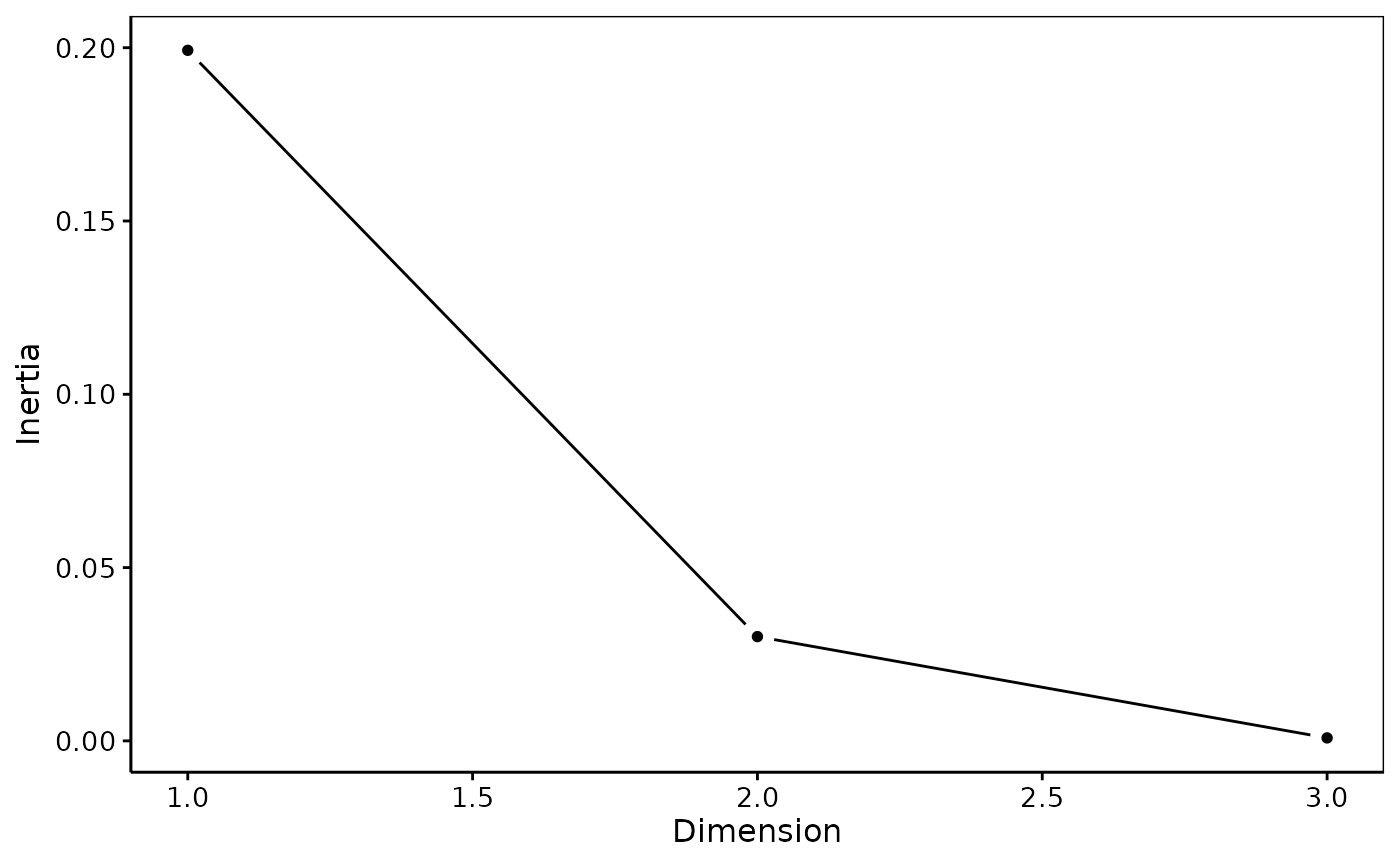
chart$altscree(caith_ca)


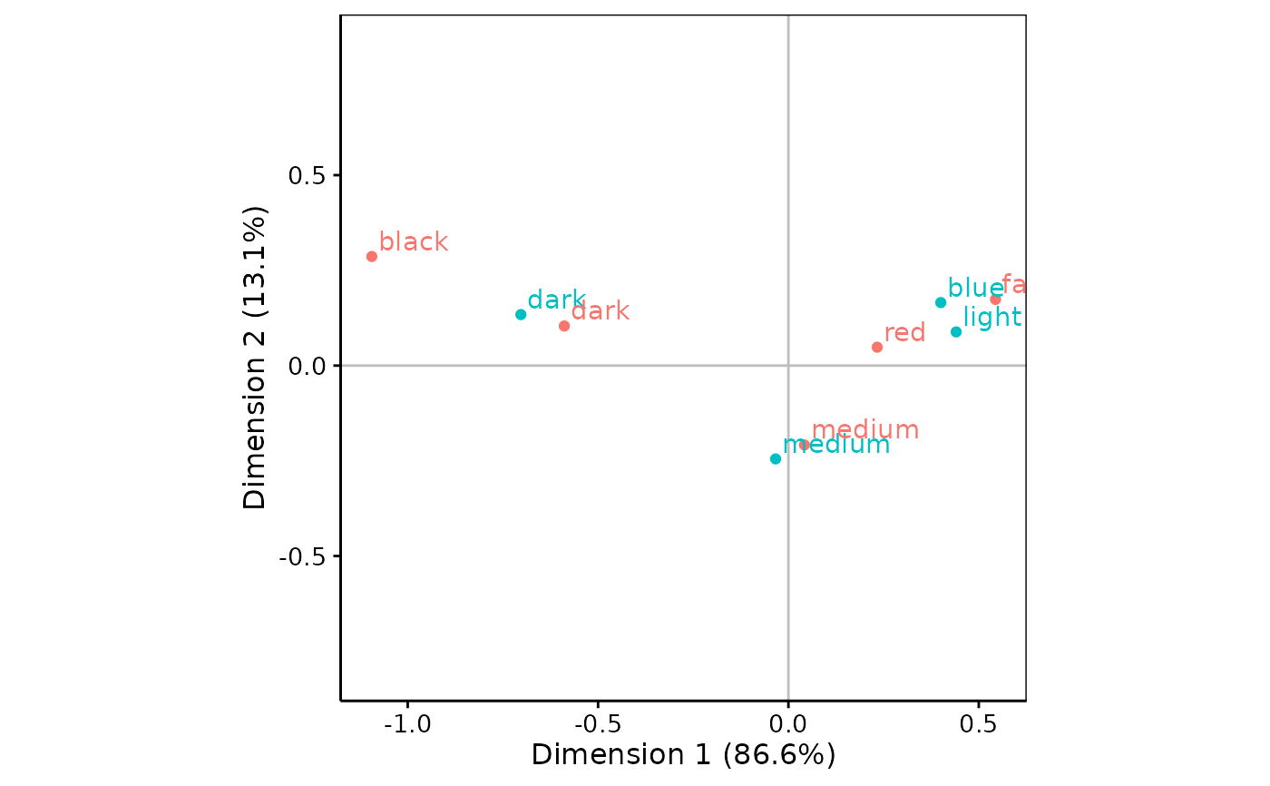
chart$biplot(caith_ca)