Principal Component Analysis (PCA)

pca(x, ...)

# S3 method for pcomp
autoplot(
  object,
  type = c("screeplot", "altscreeplot", "loadings", "correlations", "scores", "biplot"),
  choices = 1L:2L,
  name = deparse(substitute(object)),
  ar.length = 0.1,
  circle.col = "gray",
  col = "black",
  fill = "gray",
  scale = 1,
  aspect.ratio = 1,
  repel = FALSE,
  labels,
  title,
  xlab,
  ylab,
  ...
)

# S3 method for pcomp
chart(
  data,
  choices = 1L:2L,
  name = deparse(substitute(data)),
  ...,
  type = NULL,
  env = parent.frame()
)

# S3 method for princomp
augment(x, data = NULL, newdata, ...)

# S3 method for princomp
tidy(x, matrix = "u", ...)

as.prcomp(x, ...)

# S3 method for default
as.prcomp(x, ...)

# S3 method for prcomp
as.prcomp(x, ...)

# S3 method for princomp
as.prcomp(x, ...)

Arguments

x: A formula or a data frame with numeric columns, for as.prcomp(), an object to coerce into prcomp.
...: For pca(), further arguments passed to SciViews::pcomp(), notably, data= associated with a formula, subset=(optional), na.action=, method= that can be "svd" or "eigen". See SciViews::pcomp() for more details on these arguments.
object: A pcomp object
type: The type of plot to produce: "screeplot" or "altscreeplot" for two versions of the screeplot, "loadings", "correlations", or "scores" for the different views of the PCA, or a combined "biplot".
choices: Vector of two positive integers. The two axes to plot, by default first and second axes.
name: The name of the object (automatically defined by default)
ar.length: The length of the arrow head on the plot, 0.1 by default
circle.col: The color of the circle on the plot, gray by default
col: The color for the points representing the observations, black by default.
fill: The color to fill bars, gray by default
scale: The scale to apply for annotations, 1 by default
aspect.ratio: height/width of the plot, 1 by default (for plots where the ratio height / width does matter)
repel: Logical. Should repel be used to rearrange points labels? FALSEby default
labels: The label of the points (optional)
title: The title of the plot (optional, a reasonable default is used)
xlab: The label for the X axis. Automatically defined if not provided
ylab: Idem for the Y axis
data: The original data frame used for the PCA
env: The environment where to evaluate code, parent.frame() by default, which should not be changed unless you really know what you are doing!
newdata: A data frame with similar structure to data and new observations
matrix: Indicate which component should be be tidied. See broom::tidy.prcomp()

Value

pca() produces a pcomp object.

Examples

library(chart)
library(ggplot2)
data(iris, package = "datasets")
iris_num <- iris[, -5] # Only numeric columns
iris_pca <- pca(data = iris_num, ~ .)
summary(iris_pca)
#> Importance of components (eigenvalues):
#>                         PC1   PC2    PC3     PC4
#> Variance               2.92 0.914 0.1468 0.02071
#> Proportion of Variance 0.73 0.229 0.0367 0.00518
#> Cumulative Proportion  0.73 0.958 0.9948 1.00000
#> 
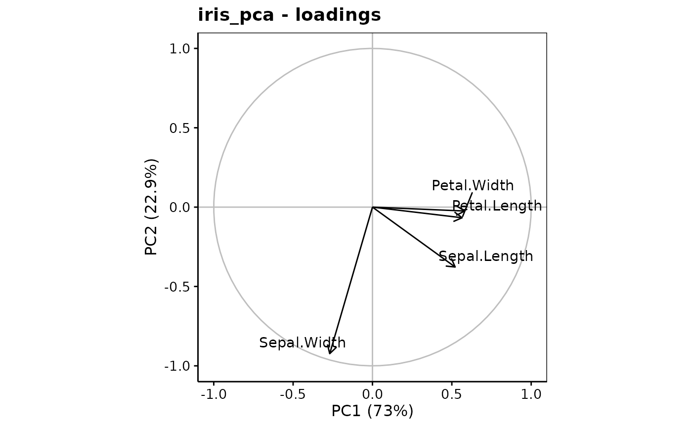
#> Loadings (eigenvectors, rotation matrix):
#>              PC1    PC2    PC3    PC4   
#> Sepal.Length  0.521 -0.377  0.720  0.261
#> Sepal.Width  -0.269 -0.923 -0.244 -0.124
#> Petal.Length  0.580        -0.142 -0.801
#> Petal.Width   0.565        -0.634  0.524
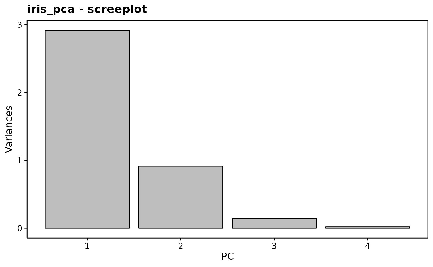
chart$scree(iris_pca) # OK to keep 2 components

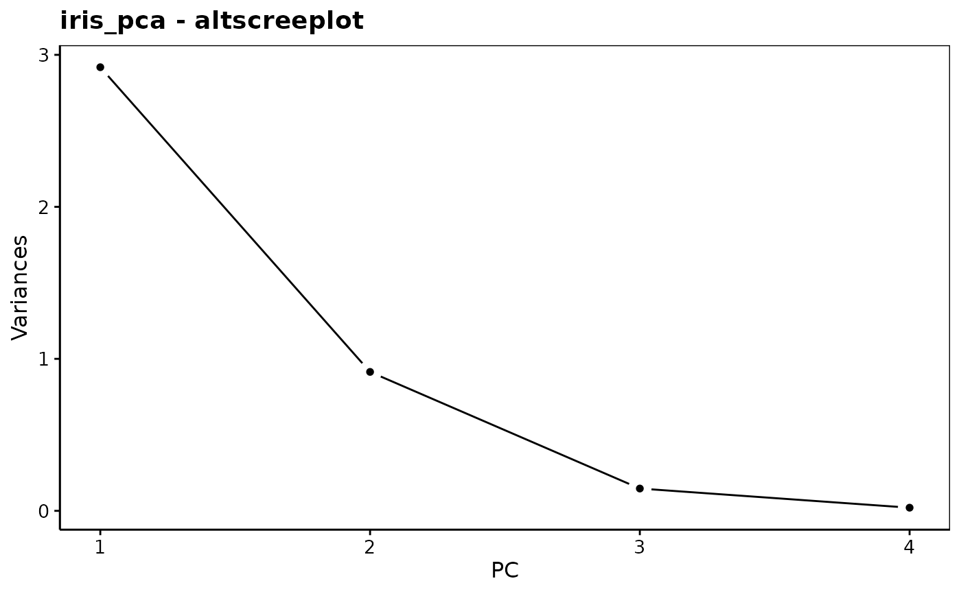
chart$altscree(iris_pca) # Different presentation


chart$loadings(iris_pca, choices = c(1L, 2L))

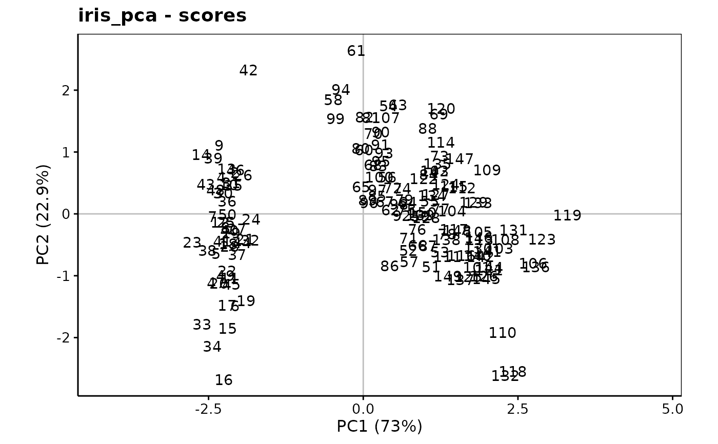
chart$scores(iris_pca, choices = c(1L, 2L), aspect.ratio = 3/5)

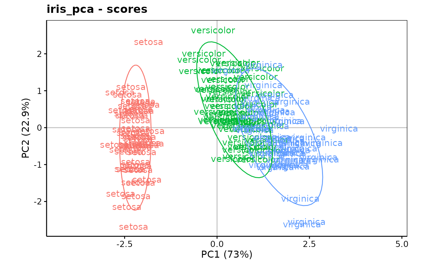
# or better:
chart$scores(iris_pca, choices = c(1L, 2L), labels = iris$Species,
  aspect.ratio = 3/5) +
  stat_ellipse()


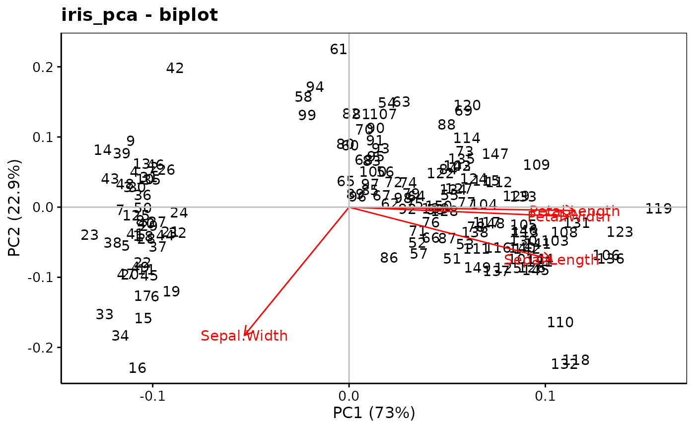
# biplot
chart$biplot(iris_pca)