‘form.io’ allows for numbering and captioning of figures, tables and equations (scientific notation) for many different R Markdown documents. LaTeX as well as the ‘bookdown’ R package provide these features, but they are limited to a set of output formats. The solution implemented in ‘form.io’ works in many places, including the default HTML, PDF and Word export formats, as well as, for R Notebooks. To experiment with it, download the present file from here, open it in RStudio, and look at the various exportation formats under the knit button.

Text with an anchor. And now, a link to it. This shows a bug with PDF: when you click on the link, the page moves up one line too high! And here is an URL: https://www.sciviews.org.

Introduction

Basic R Markdown does not allow to have numbered figures, tables and equations. The ‘bookdown’ package provides a solution that works for books. The bookdown::html_document2, bookdown::pdf_document2, bookdown::word_document2 formats activate the same extension for, respectively single-page HTML, PDF and Word outputs from standard R Markdown. There is a series of other formats in ‘bookdown’ as well, including for R Notebooks. However, users have to fiddle a little bit with the YAML header to use these formats, and the nice configuration box for the document that can be used in RStudio is not available any more. This is not something easy for a beginner.

With ‘bookdown’ the figures, tables and equations are numbered and captioned if fig.caption: yes is set in the YAML header. The numbered items can be cross-referenced by using \@ref{label}, with label being fig:... for a figure, tab:... for a table and eq:... for an equation. Figures and tables must be generated from R chunks and their labels are equivalent to the R chunk labels¹. For figures, you must provide a correctly formatted (according to the targetted output format) string in the fig.cap= argument of the chunk on a single line. The reference of a figure is fig:label where label is the corresponding label of the chunk that generated the figure. This is again not very easy for beginners, and it does not match at all the primary concept of Markdown:

A Markdown-formatted document should be publishable as-is, as plain text, without looking like it’s been marked up with tags or formatting instructions. – John Gruber

Problems are:

“Standard” R Markdown output formats do not support this feature,
Very different approaches for tables (caption= argument of knitr::kable()) and figures (fig.cap= argument of the chunk + hack required for complex captions by using so-called ‘text references’ like (ref:label) Caption defined elsewhere. together with fig.cap='(ref:foo)').
Not very easy to understand for beginners. So, it is better to skip it in an introductory course on statistics, … but what to do if we also want students to learn how to correctly write a scientific report?
The legend of tables and figures do not look like legends at all in the .Rmd file, and this is against the spirit of Markdown.

What we want:

Support for all output formats where it is pertinent (not necessarily in presentations, for instance).
Easy to set up and understand how it works.
Similar interface for figures and tables (despite it must be very different internally).
A solution that remains consistent and compatible with the ‘bookdown’ approach as much as possible, in particular for \@ref usage.
A solution that preserves the nice aspects of RStudio, like image path autocompletion, and images and equations previewing.
A layout in the .Rmd document that makes the final result obvious, something as close as possible to this:

Table: (\#tab:label) Caption of the table **with Markdown** syntax.

<code that generates the table here>

and

Figure: (\#fig:label) Caption of the figure **with Markdown** syntax.

<code that generate the display figure here>

With label being the identifier to use in \@ref(fig:label) or \@ref(tab:label) to reference it. Of course the final caption must be reworked to include a number, according to the table/figure position in the document, and the same number must be reused in the link produced by \@ref().

Our implementation, as well as, the ‘bookdown’ one cannot keep links for numbered equations. In fact, numbered equations for Word export are not supported by Pandoc, it seems. So, numbered equations are rendered with a hack that does not permit to back to them, unfortunately.

Requirements

The feature will be implemented in one of the SciViews::R package (the ‘form.io’ package looks like a natural fit). So, we need it (at the end, it would be nice to have the feature directly available after SciViews::R()).

#SciViews::R()
library(form.io)

Note that (\#tab:label), or \@ref(tab:label) will be replaced everywhere in the document, including in code blocks or R outputs! So, if you want to refer to the verbatim command, either enclose it with `, or put a marker that R will take out at the end and that breaks the pattern. That marker is -> <-.

Numbered and referenced tables

Here are twice the same tables rendered differently. Table 1 is just “enhanced” R Markdown code:

Table 1 : Ceci est la légende de ma table de `iris` et super^script en R Markdown.
First column	Second column
1	2
3	4

Table 2 is generated from within a chunk with its definition contained in an R string (or a variable, or generated by an R function), but don’t forget to set results='asis' for the chunk.

Table 2 : Ceci est la légende de ma table *générée depuis un chunk*.
First column	Second column
1	2
3	4

You see how similar these two look like in the .Rmd file? They both are in line with the Markdown philosophy to make the raw text pretty understandable what the intended formatting should be.

Why is the generated form important? Because we can use it to format various objects from within R, and output captioned and numbered tables directly. Now, I can reference the tables (Table 1 and Table 2, but also future Table 3).

Mixing online R expressions with R chunks works everywhere, except in R Notebook, because R inline expressions are not run in the editor! So, it is much better to place an Table() code (with only the caption text as argument) inside a chunk. If you don’t want to display that line of code (because you want just demonstrate nice and clean R code and after all, the table caption is part of the narration, not the code), you can put it in a distinct chunk, or better, you can put it in the chunk in first position and use echo=2:n where n is greater or equal to the number of R statements in the chunk.

form2(head(iris))

Table 3 : Ceci est une autre légende de ma table de `iris` super^script.
Sepal.Length	Sepal.Width	Petal.Length	Petal.Width	Species
5.1	3.5	1.4	0.2	setosa
4.9	3.0	1.4	0.2	setosa
4.7	3.2	1.3	0.2	setosa
4.6	3.1	1.5	0.2	setosa
5.0	3.6	1.4	0.2	setosa
5.4	3.9	1.7	0.4	setosa

Now, I can reference previous tables again (Table 1, and Table 3). Do you see how the construct remains similar in the last case? It still looks like previous constructs (although transposed in R parlance, we use the Table("table caption") code):

Table: table caption

<code that generates the table>

Here is a similar table construct, but it is not numbered because no caption is defined.

form2(head(cars))

speed	dist
4	2
4	10
7	4
7	22
8	16
9	10

Numbered and referenced display tables (2)

Another section, just to look how numbering changes from section to section…

Another table, this time in an unnamed chunk, and caption definition inside the R chunk. In this case, I can create a correct caption, but I cannot reference to it, because I don’t know the label given to it (and this is compatible with the way ‘bookdown’ behaves). Note, this time the caption is clearly visible in the code chunk because I used default value echo=TRUE in the chunk.

Table("First few lines of `trees`.")

form2(head(trees))

Table 4 : First few lines of `trees`.
Girth	Height	Volume
8.3	70	10.3
8.6	65	10.3
8.8	63	10.2
10.5	72	16.4
10.7	81	18.8
10.8	83	19.7

Finally, for all “standard” functions that have a caption= argument (or equivalent), you can provide the text caption as caption = tab("My caption text"). For instance using knitr::kable():

knitr::kable(tail(trees), caption = tab("Last few lines of `trees`."), format = "pandoc")

Table 5 : Last few lines of `trees`.
	Girth	Height	Volume
26	17.3	81	55.4
27	17.5	82	55.7
28	17.9	80	58.3
29	18.0	80	51.5
30	18.0	80	51.0
31	20.6	87	77.0

A citation of this last table (Table 5)…. and now, a simple knitr::kable() again, but note that if you don’t want to count it as a numbered table in LaTeX, you have to indicate format = 'latex' in that case, see in the.Rmd` file:

knitr::kable(tail(cars), format = if (knitr::is_latex_output()) "latex" else "pandoc")

	speed	dist
45	23	54
46	24	70
47	24	92
48	24	93
49	24	120
50	25	85

Numbered and referenced figures

The way figures are generated in R Markdown documents, and also the necessity to put the anchor for the label at the top of the figure makes things a little bit more complex. Here, we change default values for fig.cap= and out.extra= to provide at the same time a good caption and a label placed in the figure element itself. But since these are defined as default values, the end-user does not have to know these details. He just have to use Figure() function in a similar way as Table() here above.

For this demonstration, we will use an image downloaded from the internet: the R logo.

if (!file.exists("Rlogo.png"))
  download.file("https://www.r-project.org/logo/Rlogo.png", "Rlogo.png")

Figure 1 : Caption of my figure of iris from an inline r expression.

Here is a link to Fig 1 and to Fig 4. As you can see, this construct is much more suggestive (see original .Rmd file), although it has to be embedded into an R inline expression (and since ` is not allowed inside theses expressions, one can use ''' instead, like '''iris''' as equivalent to `iris`). This is pretty similar to the Table construct. Inside a R chunk, it is even more readable (but don’t forget to put results='asis' as chunk option). Inside a chunk, the figure label is automatically obtained from the chunk label, and you can use `iris`normally.

Figure 2 : Caption of my figure of iris from within an R chunk.

Of course, Figure() is compatible with knitr::include_graphics() too (But you cannot use Markdown formatting currently in the legend for LaTeX outputs, and there are other strange things, for instance, if I don’t escape the underscore, it does not work on LaTeX):

$Figure 3 : Caption of my **figure** of iris, using `include\_graphics()`.$

Figure 3 : Caption of my figure of iris, using include\_graphics().

Now, I want to display it correctly here. Theoretically, this could be done with:

![This is my caption](/private/var/folders/24/8k48jl6d249_n_qfxwsl6xvm0000gn/T/Rtmp14Sii6/fileb9cbc406fa/articles/test/test_numbering_files/figure-html/my-figure-chunk2-1.png)

… but it does not work because the document being self-contained, images are not there any more.

When you want to indicate the caption inside de chunk, but you want it to be rendered by the chunk itself (the fig.cap= property), just do provide only a single argument (the caption text). In this case, you don’t have to indicate anything in fig.cap=: a correct default value has been set up for you!

Now, one may consider the caption is not really part of the R code itself. In a tutorial, for instance, you don’t want to show the code line that generates the caption where you only want to teach how to make the plot itself. In this case, use echo=-n, where n is the number of the statement (complete R instruction) that you want to hide. Note that this does not work with R Notebook: if you put anything else than echo=TRUE there, noting is echoed! The class.source='fold-hide' might be a solution, but it does not seems to work.

iris <- read("iris", package = "datasets", lang = "fr")
chart(data = iris, sepal_length ~ petal_length %col=% species) +
  geom_point()

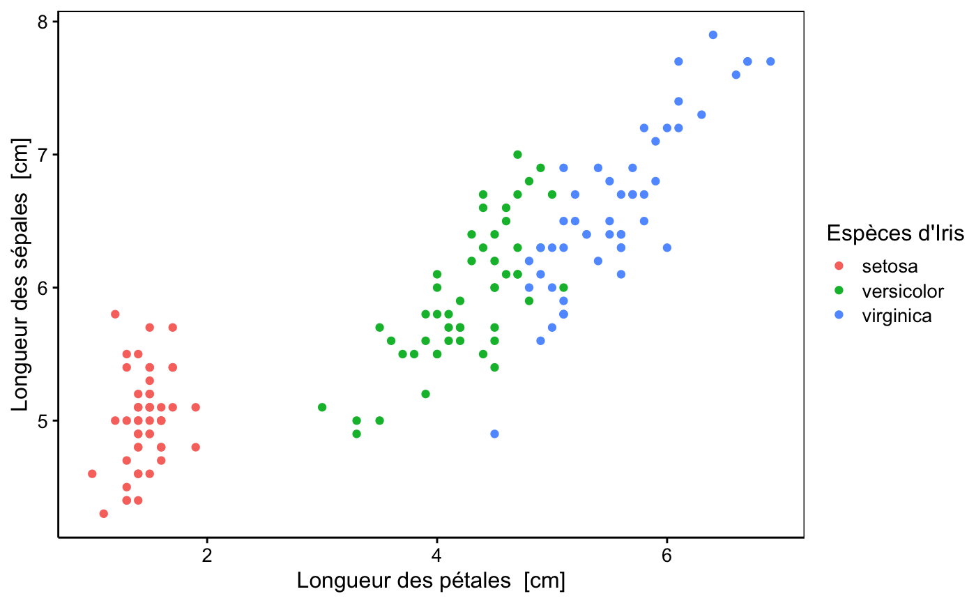
Figure 4 : Ceci est la légende de ma seconde figure.

Figure("Ceci est la légende de ma *seconde* figure.")

As you can see, the construct is flexible. You are not obliged to have the code that generates the plot just behind the Figure(...) line. Anyway, the goal of this approach is to stick with this general/overall scheme for numbered and captioned items as much as possible in all cases (R Markdown, inline R expression, or R chunks), while leaving maximum flexibility in the way your code is organized:

Figure|Table: <span id="optional-label">optional-label</span> Caption text here

<code that generate the figure or table here>

However, if you insist on using a more conventional approach by using fig.cap= instead, the new mechanism is still compatible with it… just remember to embed your caption text in fig(), which gives fig.cap=fig("My caption text"). Here is an example:

Note that this does not work in R Notebook, because it seems to ignore the fig;cap= argument!

chart(data = iris, sepal_length ~ sepal_width %col=% species) +
  geom_point()

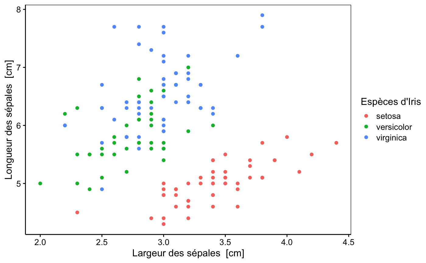
Figure 5 : My figure caption from within fig.cap= directly.

Here is again a link to Figs 1, 2, 3, Fig 4 and to Fig 5 just for verification.

Here is a link to an non-existing object: ???.

Numbered and referenced display figures (2)

Another section, just to look how numbering changes from section to section…

Here is an unnamed chunk that produces a figure, with the caption set using Figure(). In this case, the figure, the caption (and its number) are correctly rendered, but you cannot link back to the figure because you don’t know its label. If you want to display only the command that do the plot, not the Figure() part, you could indicate in the line containing it #hide#, and it will be hidden, … even in R Notebook!

chart(data = iris, sepal_length ~ species) +
  geom_boxplot()

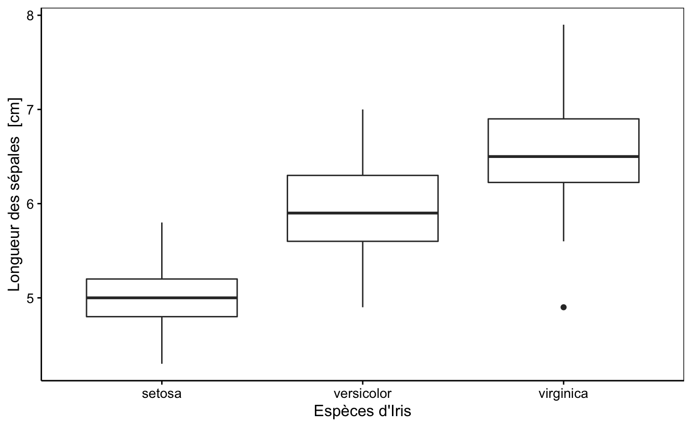
Figure 6 : Légende pour iris.

Figure("Légende pour `iris`.") #hide#

Finally, a last figure made using base plot functions, to check that the unnamed chunk figure does not mess up the succession of figures numbering:

abline(v = 1:8)
points(iris$sepal_length, iris$petal_length, col = iris$species)

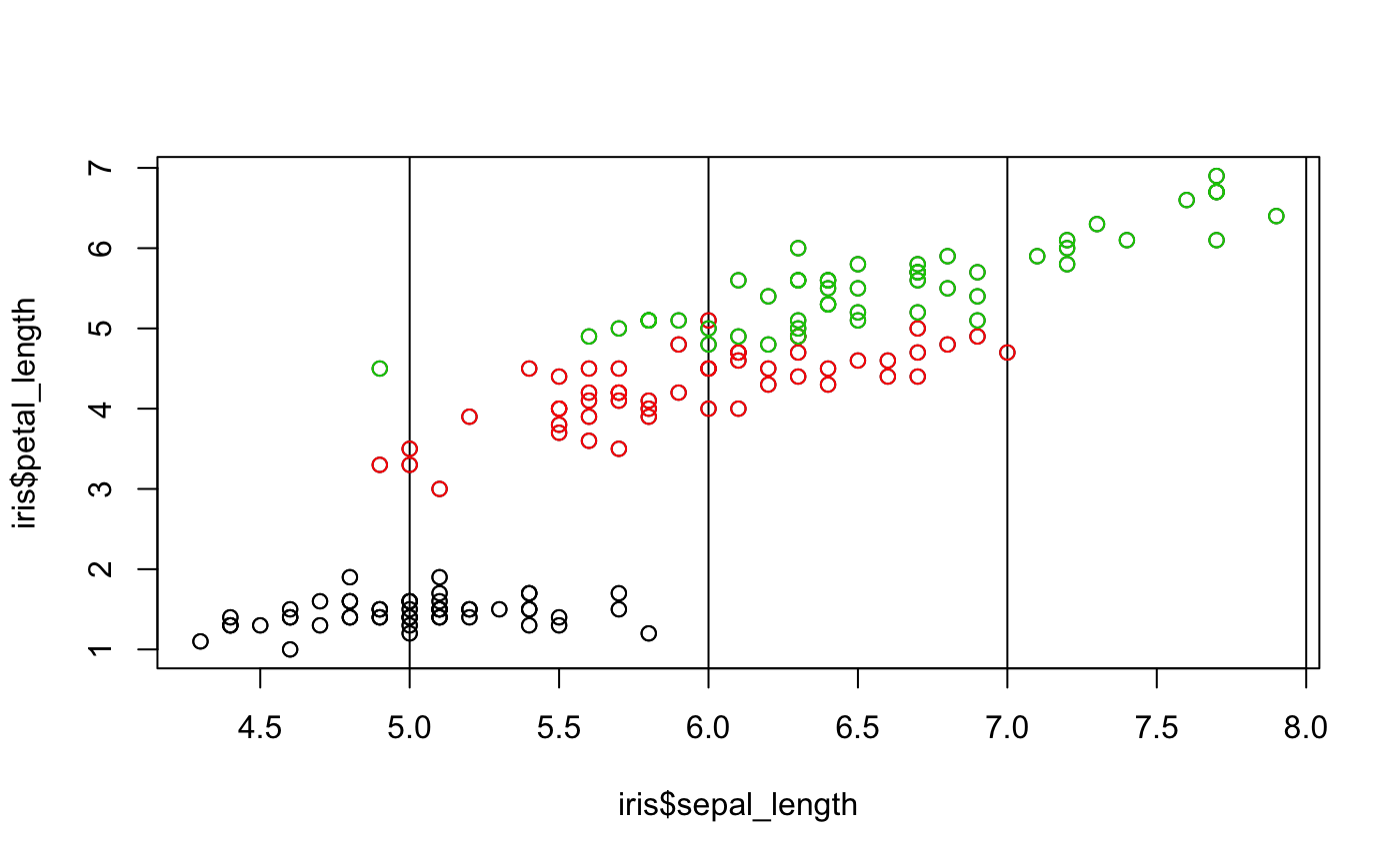
Figure 7 : Seconde légende pour iris.

Figure("Seconde légende pour `iris`.")

And now, a reference to last figure (Fig 7).

Numbered and referenced display equations

Mathjax, the engine used to manage R Markdown and Pandoc equations is able to handle this for HTML and PDF outputs, but not for Word. So, we want an alternate solution that also displays nicely in RStudio. Here it is. See in RStudio how our own implementation previews the equation with the tag set at right and with the equation label in it. This is nice to differentiate numbered and non numbered equations, and also to spot the equation label for future reference. You just have to add \tag{eq:label} at the end of your display equation, just before the final $$.

\[\sum_{i = 0}^n{x} \label{eq:sum} \tag{1} \]

Now, you can also use the ‘bookdown’ syntax ((\#eq:label)) instead, but it has to be on its own line to be compatible with ‘bookdown’, and it is less well previewed in RStudio however!

\[ \sum_{i = 0}^n{x^2} \label{eq:sumx2} \tag{2} \]

Of course, you can also cite -with links, except in Word- your numbered equations, like Eq $\eqref{eq:sum}$, or Eq $\eqref{eq:sumx2}$, or Eq $\eqref{eq:pythagoras}$.

\[a^2+b^2=c^2 \label{eq:pythagoras} \tag{3} \]

TODO

Different color for links in LaTeX (hyperref argument)
Place Figure;/Figure() beneath the code that generates the figure
Allow to choose between and with the later one by default for compatibility with ‘bookdown’.
Force numbered captioned figures even when fig_caption: no (default) is used.
allow a multiline text in Figure() and Table()
Put all this code in the ‘form.io’ package
labels in ‘bookdown’ are only -/a-zA-Z0-9 (what about accented characters?) and we should choose something else for word separation, e.g., -, with /- being - itself
R Notebook: certain table or figure labels are not resolved (missing \ in (\#...)) + avoid the ugly and inconvenient table preview in RStudio
PDF document: figures using knitr::includegraphics incorrect + avoid duplication of Figure/Table header + non-captioned tables increment too.
bookdown::pdf_document2: equations incorrect + knitr::include_graphics() do not work. Links to figures link to legend, and not the image. Do not use pandoc format in knitr::kable() for non captioned tables.
Word: Format numbered equations + links to figures do not work
knitr::include_graphics(, auto_pdf = TRUE) replaces .png by .pdf if the latter file exists and output to LaTeX for a better final result, and it can be activated globally by options(knitr.graphics.auto_pdf = TRUE) => make the same for our figures
Allow for enhanced R Markdown style Figure:...\n\n![]() + tab.cap= and other stuff in R chunks
explore printr, kableExtra, gt, pander, xtable, tables, syPlot::sjt*
center figures and tables by defaut + allow customization general and particular
fig.pos=“H” for LaTeX, see https://stackoverrun.com/fr/q/8164644
on a different topic: make citation text smaller, document hook for bibliography compilation and to insert sessionInfo, and dark mode.

Bugs and shortcomings

When knitting to Word document (either standard, or ‘bookdown’ version), there is no links to Tables, Figures or equations.
Links to figures generated from R chunks in the traditional PDF format does not work yet (the ‘bookdown’ version is operational).
Captions from R chunks for LaTeX outputs do not interpret Markdown formatting yet. Also, you must escape special characters like _, or it will not be rendered correctly.
Equations numbering in the ‘bookdown’ version of PDF seems to be buggy.
With R Notebook and LaTeX, links to figures actually ling to first line of the caption. This is also true for the ‘bookdown’ version of PDF.
With R notebook, there my be a line of code between the figure and its caption (use echo=FALSE to avoid it).
The fig.cap= chunk option is not used by R Notebook. So, it is not possible to generate caption this way in that case. For maximum compatibility, always use the Figure() code in the chunk itself.
The R Notebook format does not recognizes the echo=n version. If echo is not set to TRUE, it displays just nothing.
Placement and size of table and figures differ from one to the other format. We have not yet worked that aspect for a more homogeneous result.
It is currently obligatory to indicate fig_caption:yes explicitly in HTML and Word documents to have the figure captions actually rendered (we plan another solution).
In the ‘bookdown’ version of the Word document, numbered equations are wrongly labelled with their name. In the plain Word version, it is correct.

Miscellaneous

Différentes choses trouvées au fur et à mesure du développement de ce truc!

Il est possible d’ajouter le numéro de chapitre a posteriori en CSS avec quelque chose comme:

Rien à voir, mais voici peut-être une solution pour les documents multi-languages… et pour des sections optionnelles! Mais sont-elles réellement absentes du document? Et il faudrait implementer aussi ceci en LaTeX et Word. Le mieux serait d’avoir une balise spécifique traitée directement depuis R…

This is a section in English. I want the French part as close as possible to it.

Ceci est une section en français. Je veux la partie anglaise aussi proche que possible de celui-ci.

TODO: Un g(...) utilisant glue() pour les inline expressions pour faciliter la generation d’items à partir de R.

Ceci est un ‘line_block’
Je me demande ce que ça donne
en sortie…?

Task lists work only in the Github markdown format.

Item 1
Item 2

Knitr hooks work like this:

knitr::knit_hooks$set(error = function(x, options) {
  paste(c('\n\n:::{style="color:Crimson; background-color: SeaShell;"}',
        gsub('^#> Error', '**Error**', x),
        ':::'), collapse = '\n')
})

You may test the hook with a code chunk like this:

1 + "a"

Error in 1 + “a”: non-numeric argument to binary operator

To get a list of (main) options for the current R Markdown output format (except html_notebook), place a chunk in your document with this code. But in an R Notebook you got an error, so catch it!

res <- try(rmarkdown::default_output_format(knitr::current_input()), silent = TRUE)
if (inherits(res, "try-error")) NULL else res

#> $name
#> [1] "html_document"
#> 
#> $options
#> $options$toc
#> [1] FALSE
#> 
#> $options$toc_depth
#> [1] 3
#> 
#> $options$toc_float
#> [1] FALSE
#> 
#> $options$number_sections
#> [1] FALSE
#> 
#> $options$section_divs
#> [1] TRUE
#> 
#> $options$fig_width
#> [1] 7
#> 
#> $options$fig_height
#> [1] 5
#> 
#> $options$fig_retina
#> [1] 2
#> 
#> $options$dev
#> [1] "png"
#> 
#> $options$df_print
#> [1] "default"
#> 
#> $options$smart
#> [1] TRUE
#> 
#> $options$self_contained
#> [1] TRUE
#> 
#> $options$theme
#> [1] "default"
#> 
#> $options$highlight
#> [1] "default"
#> 
#> $options$mathjax
#> [1] "default"
#> 
#> $options$template
#> [1] "default"
#> 
#> $options$extra_dependencies
#> NULL
#> 
#> $options$css
#> NULL
#> 
#> $options$includes
#> NULL
#> 
#> $options$lib_dir
#> NULL
#> 
#> $options$md_extensions
#> NULL
#> 
#> $options$pandoc_args
#> NULL
#> 
#> $options$...
#> 
#> 
#> $options$code_folding
#> [1] "show"
#> 
#> $options$code_download
#> [1] TRUE
#> 
#> $options$fig_caption
#> [1] TRUE
#> 
#> $options$keep_md
#> [1] FALSE
#> 
#> $options$bookdown
#> [1] FALSE

Numbered tables can also be generated with a header line like Table: (\#tab:label) Caption.↩︎

Test of figures, tables and equations numbering

Philippe Grosjean (phgrosjean@sciviews.org)

2020-04-25