Create and plot density functions for distribution objects

The distribution objects represent one or more statistical distributions. The functions dfun() and geom_funfill(), together with chart() allow to plot them.

dfun(object, i = 1)

cdfun(object, i = 1)

# S3 method for class 'distribution'
autoplot(
  object,
  n = 500,
  xlim = NULL,
  size = 99.5,
  xlab = "Quantile",
  ylab = if (type == "density") "Probability density" else
    "Cumulative probability density",
  plot.it = TRUE,
  use.chart = FALSE,
  ...,
  type = "density",
  theme = NULL
)

# S3 method for class 'distribution'
chart(data, ..., type = "density", env = parent.frame())

geom_funfill(
  mapping = NULL,
  data = NULL,
  fun,
  from,
  to,
  geom = "area",
  fill = "salmon",
  alpha = 0.5,
  ...
)

Arguments

object: A distribution object, as from the {distributional} package.
i: The distribution to use from the list (first one by default)
n: The number of points to use to draw the density functions (500 by default) of continuous distributions.
xlim: Two numbers that limit the X axis.
size: If xlim= is not provided, it is automatically calculated using the size of the CI between 0 and 100 (99.5 by default) for continuous distributions.
xlab: The label of the X axis ("Quantile" by default).
ylab: The label of the Y axis ("Probability density" or "Cumulative probability density" by default).
plot.it: Should the densities be plotted for all the distributions (TRUE by default)?
use.chart: Should chart() be used (TRUE by default)? Otherwise, ggplot() is used.
...: Further arguments to stat_function().
type: The type of plot ("density" by default, or "cumulative").
theme: The theme for the plot (ignored for now).
data: The data frame to use (NULL by default).
env: The environment to use to evaluate expressions.
mapping: the mapping to use (NULL by default.
fun: The function to use (could be dfun(distribution_object)).
from: The first quantile to delimit the filled area.
to: The second quantile to delimit the filled area.
geom: The geom to use ("area" by default).
fill: The color to fill the area ("salmon" by default).
alpha: The alpha transparency to apply, 0.5 by default.

Value

Either a function or a ggplot object.

Examples

library(distributional)
library(chart)
#> Loading required package: ggplot2
#> Loading required package: lattice
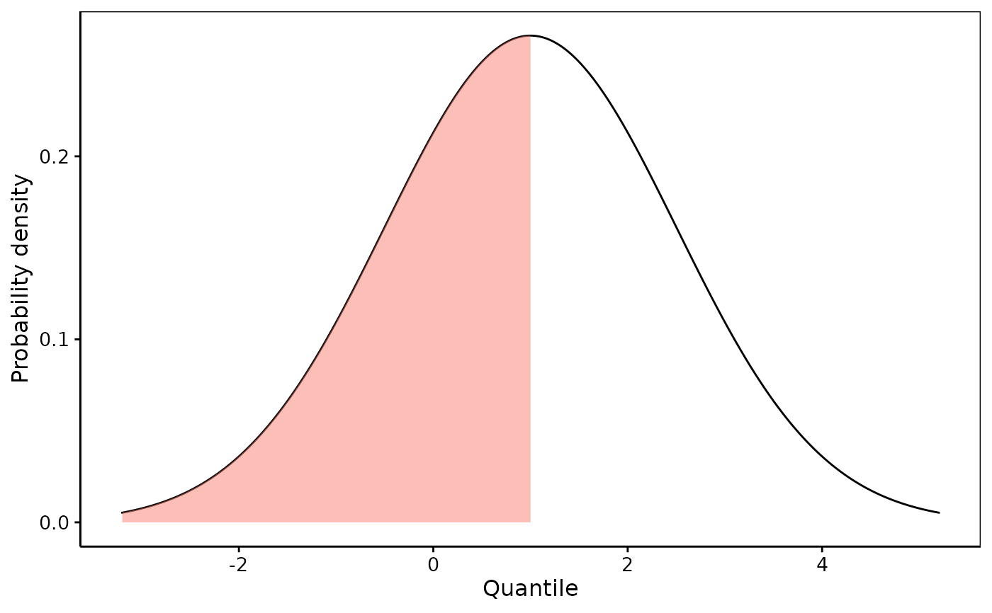
di1 <- dist_normal(mu = 1, sigma = 1.5)
chart(di1) +
  geom_funfill(fun = dfun(di1), from = -5, to = 1)


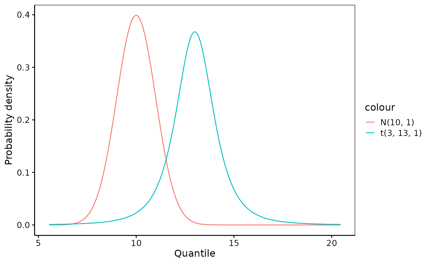
# With two distributions
di2 <- c(dist_normal(10, 1), dist_student_t(df = 3, 13, 1))
chart(di2) +
  geom_funfill(fun = dfun(di2, 1), from = -5, to = 0) +
  geom_funfill(fun = dfun(di2, 2), from = 2, to = 6, fill = "turquoise3")
#> Warning: no non-missing arguments to max; returning -Inf

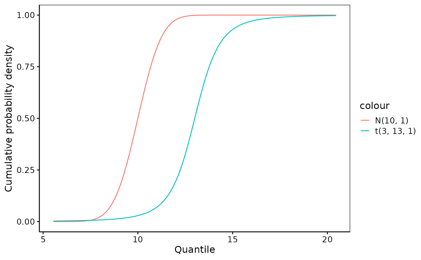
chart$cumulative(di2)

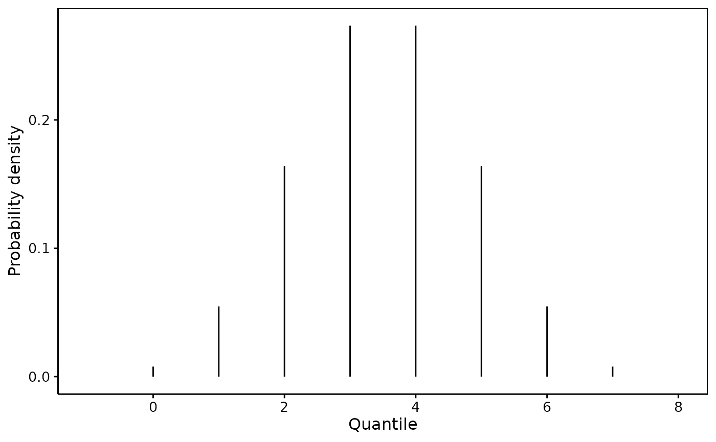
# A discrete distribution
di3 <- dist_binomial(size = 7, prob = 0.5)
chart(di3)

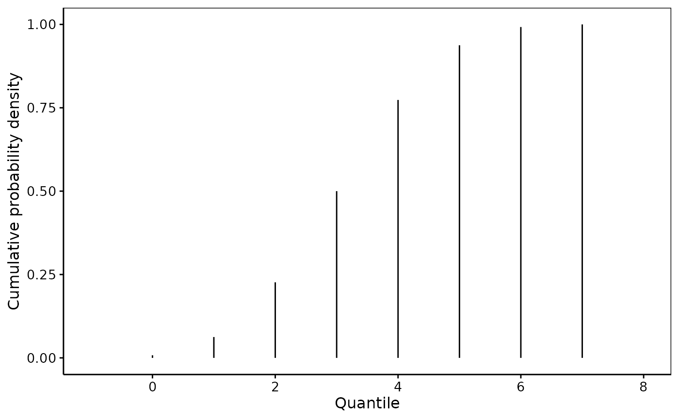
chart$cumulative(di3)

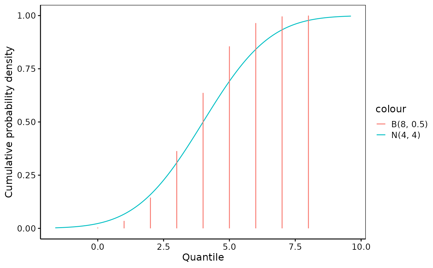
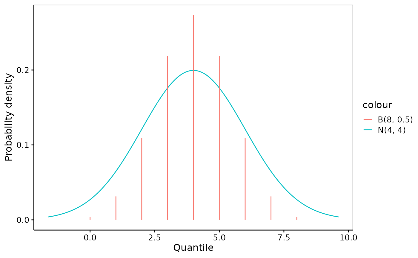
# A continuous together with a discrete distribution
di4 <- c(dist_normal(mu = 4, sigma = 2), dist_binomial(size = 8, prob = 0.5))
chart(di4)

chart$cumulative(di4)