Create a rich-formatted table from the summary of a nls object

Create a table of a summary.nls object. This table looks like the output of print.summary.nls() but richly formatted. The tabularise_coef() function offers more customization options for this object.

# S3 method for class 'summary.nls'
tabularise_default(
  data,
  header = TRUE,
  title = header,
  equation = header,
  auto.labs = TRUE,
  origdata = NULL,
  labs = NULL,
  lang = getOption("SciViews_lang", "en"),
  footer = TRUE,
  show.signif.stars = getOption("show.signif.stars", TRUE),
  ...,
  kind = "ft"
)

Arguments

data: An nls object.
header: If TRUE (by default), add a title to the table.
title: If TRUE, add a title to the table header. Default to the same value than header, except outside of a chunk where it is FALSE if a table caption is detected (tbl-cap YAML entry).
equation: Add equation of the model to the table. If TRUE, equation() is used. The equation can also be passed in the form of a character string (LaTeX).
auto.labs: If TRUE (by default), use labels (and units) automatically from data or origdata=.
origdata: The original data set this model was fitted to. By default it is NULL and no label is used (only the name of the variables).
labs: Labels to change the names of elements in the term column of the table. By default it is NULL and nothing is changed.
lang: The language to use. The default value can be set with, e.g., options(SciViews_lang = "fr") for French.
footer: If TRUE (by default), add a footer to the table.
show.signif.stars: If TRUE, add the significance stars to the table. The default is getOption("show.signif.stars")
...: Not used
kind: The kind of table to produce: "tt" for tinytable, or "ft" for flextable (default).

Value

A flextable object that you can print in different forms or rearrange with the {flextable} functions.

Examples

data("ChickWeight", package = "datasets")
chick1 <- ChickWeight[ChickWeight$Chick == 1, ]

# Adjust a logistic curve
chick1_logis <- nls(data = chick1, weight ~ SSlogis(Time, Asym, xmid, scal))
chick1_logis_sum <- summary(chick1_logis)

tabularise::tabularise(chick1_logis_sum)
Nonlinear least squares  logistic model
 $\begin{aligned} \operatorname{weight} = \frac{Asym}{1 + e^{(xmid - \operatorname{Time}) /scal}} + \epsilon \end{aligned}$ 
Term Estimate Standard Error tobs. value p value signif
Asym 937.0 465.868  2.01 7.52·10-02   .
xmid  35.2   8.312  4.24 2.18·10-03  **
scal  11.4   0.905 12.60 5.08·10-07 ***
0 <= '***' < 0.001 < '**' < 0.01 < '*' < 0.05
Residuals standard error: 2.919 on 9 degrees of freedom
Number of iterations to convergence: 0
Achieved convergence tolerance: 7.343e-06
tabularise::tabularise(chick1_logis_sum, footer = FALSE)
Nonlinear least squares  logistic model
 $\begin{aligned} \operatorname{weight} = \frac{Asym}{1 + e^{(xmid - \operatorname{Time}) /scal}} + \epsilon \end{aligned}$ 
Term Estimate Standard Error tobs. value p value signif
Asym 937.0 465.868  2.01 7.52·10-02   .
xmid  35.2   8.312  4.24 2.18·10-03  **
scal  11.4   0.905 12.60 5.08·10-07 ***
0 <= '***' < 0.001 < '**' < 0.01 < '*' < 0.05

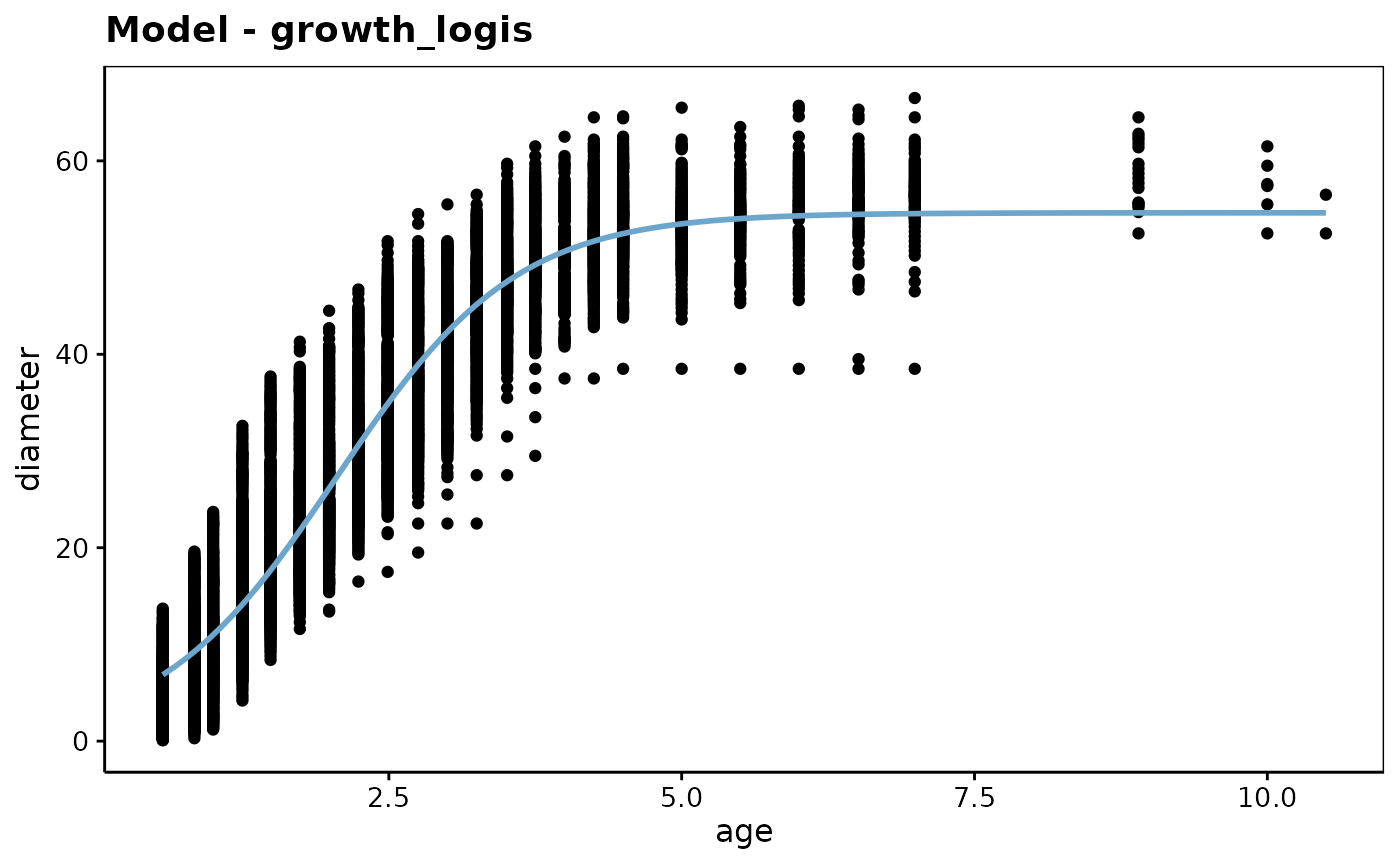
growth <- data.io::read("urchin_growth", package = "data.io")
growth_logis <- nls(data = growth, diameter ~ SSlogis(age, Asym, xmid, scal))
chart::chart(growth_logis)

tabularise::tabularise(summary(growth_logis)) # No labels
Nonlinear least squares  logistic model
 $\begin{aligned} \operatorname{diameter} = \frac{Asym}{1 + e^{(xmid - \operatorname{age}) /scal}} + \epsilon \end{aligned}$ 
Term Estimate Standard Error tobs. value p value signif
Asym 54.628 0.20299 269 < 2·10-16 ***
xmid  2.055 0.00957 215 < 2·10-16 ***
scal  0.765 0.00735 104 < 2·10-16 ***
0 <= '***' < 0.001 < '**' < 0.01 < '*' < 0.05
Residuals standard error: 5.6 on 7021 degrees of freedom
Number of iterations to convergence: 4
Achieved convergence tolerance: 1.079e-06
tabularise::tabularise(summary(growth_logis), origdata = growth) # with labels
Nonlinear least squares  logistic model
 $\begin{aligned} \operatorname{Test \ diameter \ \ [mm]} = \frac{Asym}{1 + e^{(xmid - \operatorname{Age \ \ [years]}) /scal}} + \epsilon \end{aligned}$ 
Term Estimate Standard Error tobs. value p value signif
Asym 54.628 0.20299 269 < 2·10-16 ***
xmid  2.055 0.00957 215 < 2·10-16 ***
scal  0.765 0.00735 104 < 2·10-16 ***
0 <= '***' < 0.001 < '**' < 0.01 < '*' < 0.05
Residuals standard error: 5.6 on 7021 degrees of freedom
Number of iterations to convergence: 4
Achieved convergence tolerance: 1.079e-06
tabularise::tabularise(summary(growth_logis), origdata = growth,
  equation = FALSE, show.signif.stars = FALSE)
Nonlinear least squares  logistic model
Term Estimate Standard Error tobs. value p value
Asym 54.628 0.20299 269 < 2·10-16
xmid  2.055 0.00957 215 < 2·10-16
scal  0.765 0.00735 104 < 2·10-16
Residuals standard error: 5.6 on 7021 degrees of freedom
Number of iterations to convergence: 4
Achieved convergence tolerance: 1.079e-06

Nonlinear least squares logistic model
$\begin{aligned} \operatorname{weight} = \frac{Asym}{1 + e^{(xmid - \operatorname{Time}) /scal}} + \epsilon \end{aligned}$
Term	Estimate	Standard Error	tobs. value	p value	signif
Asym	937.0	465.868	2.01	7.52·10-02	.
xmid	35.2	8.312	4.24	2.18·10-03	**
scal	11.4	0.905	12.60	5.08·10-07	***
0 <= '*' < 0.001 < '' < 0.01 < '*' < 0.05
Residuals standard error: 2.919 on 9 degrees of freedom
Number of iterations to convergence: 0 Achieved convergence tolerance: 7.343e-06

Nonlinear least squares logistic model
$\begin{aligned} \operatorname{diameter} = \frac{Asym}{1 + e^{(xmid - \operatorname{age}) /scal}} + \epsilon \end{aligned}$
Term	Estimate	Standard Error	tobs. value	p value	signif
Asym	54.628	0.20299	269	< 2·10-16	***
xmid	2.055	0.00957	215	< 2·10-16	***
scal	0.765	0.00735	104	< 2·10-16	***
0 <= '*' < 0.001 < '' < 0.01 < '*' < 0.05
Residuals standard error: 5.6 on 7021 degrees of freedom
Number of iterations to convergence: 4 Achieved convergence tolerance: 1.079e-06

Nonlinear least squares logistic model
$\begin{aligned} \operatorname{Test \ diameter \ \ [mm]} = \frac{Asym}{1 + e^{(xmid - \operatorname{Age \ \ [years]}) /scal}} + \epsilon \end{aligned}$
Term	Estimate	Standard Error	tobs. value	p value	signif
Asym	54.628	0.20299	269	< 2·10-16	***
xmid	2.055	0.00957	215	< 2·10-16	***
scal	0.765	0.00735	104	< 2·10-16	***
0 <= '*' < 0.001 < '' < 0.01 < '*' < 0.05
Residuals standard error: 5.6 on 7021 degrees of freedom
Number of iterations to convergence: 4 Achieved convergence tolerance: 1.079e-06

Arguments

Value

See also

Examples