AutoD2, CrossD2 or CenterD2 analysis of a multiple time-series

Compute and plot multiple autocorrelation using Mahalanobis generalized distance D2. AutoD2 uses the same multiple time-series. CrossD2 compares two sets of multiple time-series having same size (same number of descriptors). CenterD2 compares subsamples issued from a single multivariate time-series, aiming to detect discontinuities.

AutoD2(series, lags=c(1, nrow(series)/3), step=1, plotit=TRUE,
        add=FALSE, ...)
CrossD2(series, series2, lags=c(1, nrow(series)/3), step=1,
        plotit=TRUE, add=FALSE, ...)
CenterD2(series, window=nrow(series)/5, plotit=TRUE, add=FALSE,
        type="l", level=0.05, lhorz=TRUE, lcol=2, llty=2, ...)

Arguments

series: regularized multiple time-series
series2: a second set of regularized multiple time-series
lags: minimal and maximal lag to use. By default, 1 and a third of the number of observations in the series respectively
step: step between successive lags. By default, 1
window: the window to use for CenterD2. By default, a fifth of the total number of observations in the series
plotit: if TRUE then also plot the graph
add: if TRUE then the graph is added to the current figure
type: The type of line to draw in the CenterD2 graph. By default, a line without points
level: The significance level to consider in the CenterD2 analysis. By default 5%
lhorz: Do we have to plot also the horizontal line representing the significance level on the graph?
lcol: The color of the significance level line. By default, color 2 is used
llty: The style for the significance level line. By default: llty=2, a dashed line is drawn
...: additional graph parameters

Value

An object of class 'D2' which contains:

lag: The vector of lags
D2: The D2 value for this lag
call: The command invoked when this function was called
data: The series used
type: The type of 'D2' analysis: 'AutoD2', 'CrossD2' or 'CenterD2'
window: The size of the window used in the CenterD2 analysis
level: The significance level for CenterD2
chisq: The chi-square value corresponding to the significance level in the CenterD2 analysis
units.text: Time units of the series, nicely formatted for graphs

References

Cooley, W.W. & P.R. Lohnes, 1962. Multivariate procedures for the behavioral sciences. Whiley & sons.

DagnÃ©lie, P., 1975. Analyse statistique ? plusieurs variables. Presses Agronomiques de Gembloux.

Ibanez, F., 1975. Contribution Ã l'analyse mathÃ©matique des Ã©vÃ¨nements en Ã©cologie planctonique: optimisations mÃ©thodologiques; Ã©tude expÃ©rimentale en continu Ã petite Ã©chelle du plancton cÃ´tier. ThÃ¨se d'Ã©tat, Paris VI.

Ibanez, F., 1976. Contribution Ã l'analyse mathÃ©matique des Ã©vÃ¨nements en Ã©cologie planctonique. Optimisations mÃ©thodologiques. Bull. Inst. OcÃ©anogr. Monaco, 72:1-96.

Ibanez, F., 1981. Immediate detection of heterogeneities in continuous multivariate oceanographic recordings. Application to time series analysis of changes in the bay of Villefranche sur mer. Limnol. Oceanogr., 26:336-349.

Ibanez, F., 1991. Treatment of the data deriving from the COST 647 project on coastal benthic ecology: The within-site analysis. In: B. Keegan (ed), Space and time series data analysis in coastal benthic ecology, p 5-43.

Author

WARNING

If data are too heterogeneous, results could be biased (a singularity matrix appears in the calculations).

Examples

data(marphy)
marphy.ts <- as.ts(as.matrix(marphy[, 1:3]))
AutoD2(marphy.ts)

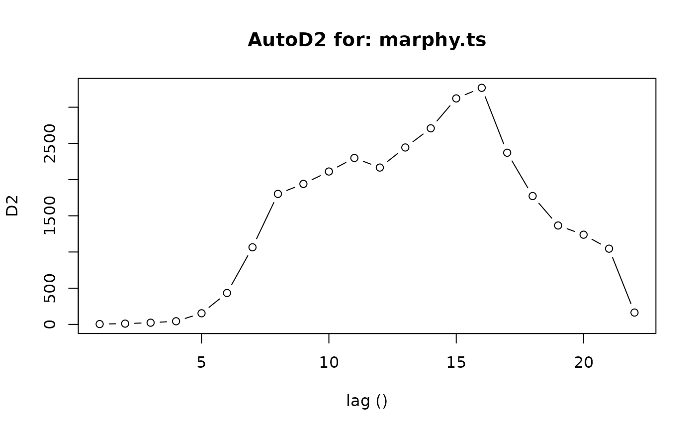#> $lag
#>  [1]  1  2  3  4  5  6  7  8  9 10 11 12 13 14 15 16 17 18 19 20 21 22
#> 
#> $D2
#>  [1]    4.22573   10.58976   23.47267   43.38305  153.44283  433.54182
#>  [7] 1064.54132 1802.43083 1940.63240 2111.62737 2298.56609 2166.24216
#> [13] 2443.59445 2708.61304 3121.54365 3267.95116 2370.99649 1772.94559
#> [19] 1366.08938 1239.05153 1045.82545  163.43575
#> 
#> $call
#> AutoD2(series = marphy.ts)
#> 
#> $data
#> [1] "marphy.ts"
#> 
#> $type
#> [1] "AutoD2"
#> 
#> $units.text
#> [1] ""
#> 
#> attr(,"class")
#> [1] "D2"
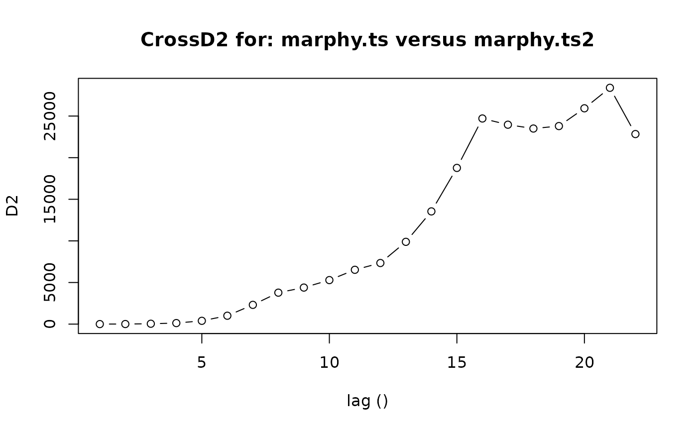
marphy.ts2 <- as.ts(as.matrix(marphy[, c(1, 4, 3)]))
CrossD2(marphy.ts, marphy.ts2)

#> $lag
#>  [1]  1  2  3  4  5  6  7  8  9 10 11 12 13 14 15 16 17 18 19 20 21 22
#> 
#> $D2
#>  [1]     4.323043    10.155231    45.764444   124.524831   395.341890
#>  [6]  1008.216533  2314.110604  3780.247450  4391.117099  5289.482066
#> [11]  6527.234759  7341.803004  9887.267753 13544.128938 18768.866938
#> [16] 24708.252337 23961.156382 23500.686505 23796.894859 25932.921344
#> [21] 28394.452862 22836.606581
#> 
#> $call
#> CrossD2(series = marphy.ts, series2 = marphy.ts2)
#> 
#> $data
#> [1] "marphy.ts"
#> 
#> $data2
#> [1] "marphy.ts2"
#> 
#> $type
#> [1] "CrossD2"
#> 
#> $units.text
#> [1] ""
#> 
#> attr(,"class")
#> [1] "D2"
# This is not identical to:
CrossD2(marphy.ts2, marphy.ts)

#> $lag
#>  [1]  1  2  3  4  5  6  7  8  9 10 11 12 13 14 15 16 17 18 19 20 21 22
#> 
#> $D2
#>  [1]   30.76921   62.83820  112.50639  215.13122  475.90799  979.41968
#>  [7] 1907.94064 2927.17901 3434.67167 4209.00250 4918.96322 5091.38349
#> [13] 5842.69358 6713.53204 7942.49390 8759.94122 7834.21656 7034.27185
#> [19] 6140.98599 5689.15330 5334.47184 3841.11059
#> 
#> $call
#> CrossD2(series = marphy.ts2, series2 = marphy.ts)
#> 
#> $data
#> [1] "marphy.ts2"
#> 
#> $data2
#> [1] "marphy.ts"
#> 
#> $type
#> [1] "CrossD2"
#> 
#> $units.text
#> [1] ""
#> 
#> attr(,"class")
#> [1] "D2"
marphy.d2 <- CenterD2(marphy.ts, window=16)
lines(c(17, 17), c(-1, 15), col=4, lty=2)
lines(c(25, 25), c(-1, 15), col=4, lty=2)
lines(c(30, 30), c(-1, 15), col=4, lty=2)
lines(c(41, 41), c(-1, 15), col=4, lty=2)
lines(c(46, 46), c(-1, 15), col=4, lty=2)
text(c(8.5, 21, 27.5, 35, 43.5, 57), 11, labels=c("Peripheral Zone", "D1",
        "C", "Front", "D2", "Central Zone")) # Labels

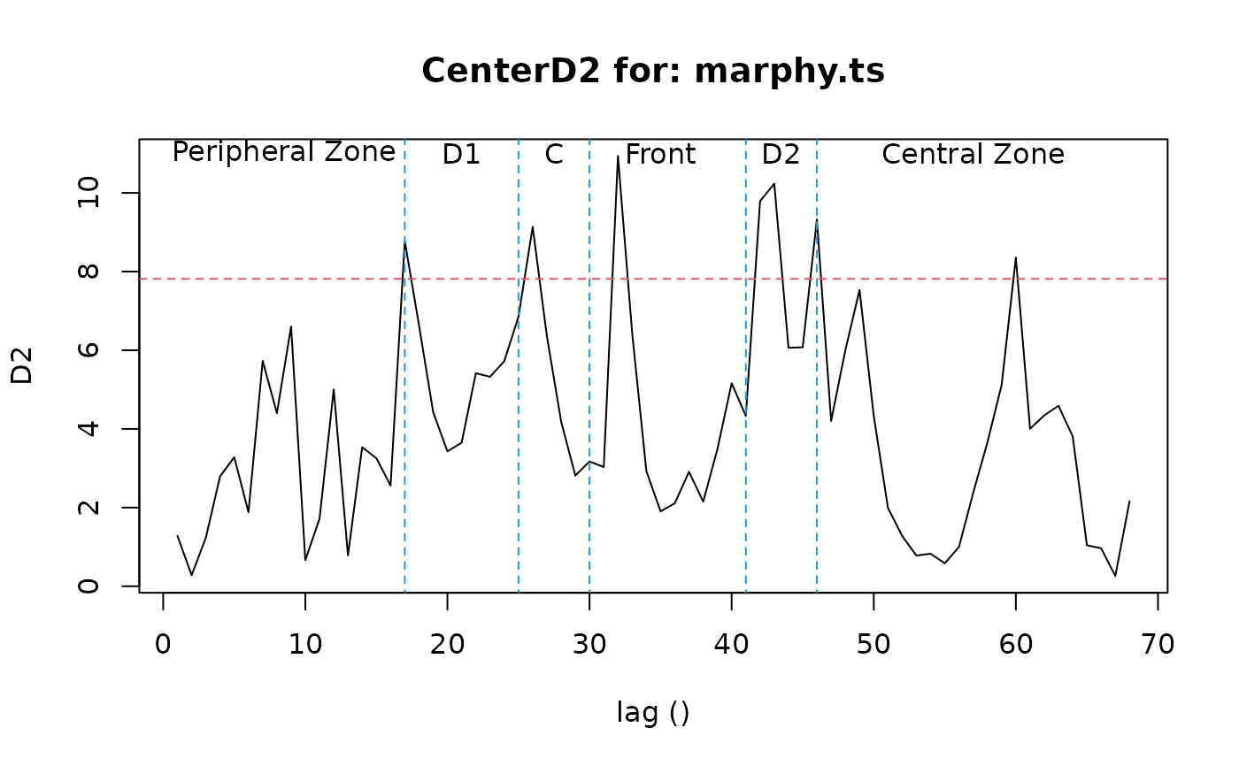time(marphy.ts)[marphy.d2$D2 > marphy.d2$chisq]
#> [1] 17 26 32 42 43 46 60