
Sort variables by abundance
abund.RdSort variables (usually species in a species x stations matrix) in function of
their abundance, either in number of non-null values, or in number of
individuals (in log). The f coefficient allows adjusting weight given to each of these two criteria.
abund(x, f = 0.2)
# S3 method for class 'abund'
extract(e, n, left = TRUE, ...)
# S3 method for class 'abund'
identify(x, label.pts = FALSE, lvert = TRUE, lvars = TRUE, col = 2, lty = 2, ...)
# S3 method for class 'abund'
lines(x, n = x$n, lvert = TRUE, lvars = TRUE, col = 2, lty = 2, ...)
# S3 method for class 'abund'
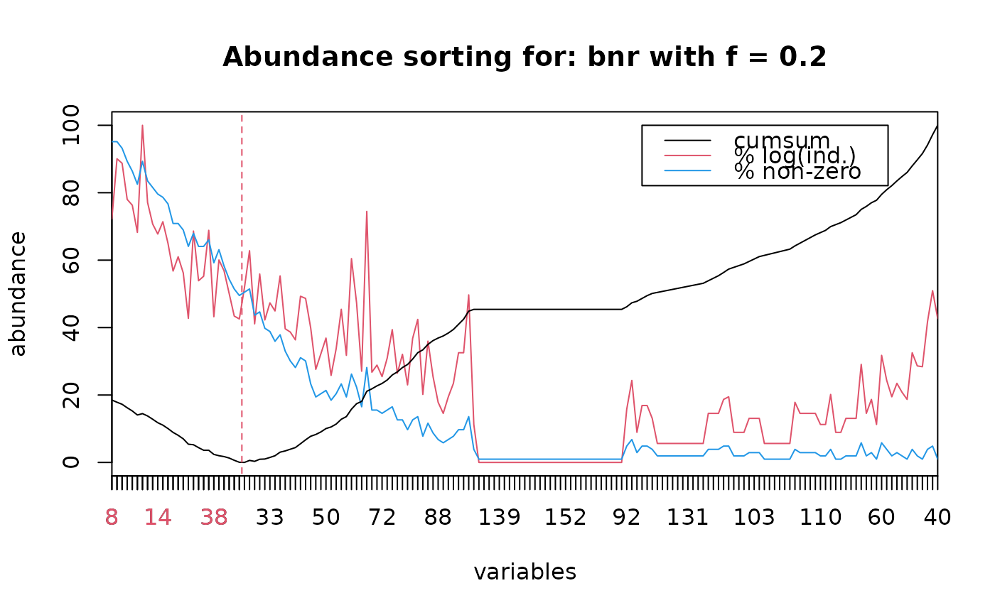
plot(x, n = x$n, lvert = TRUE, lvars = TRUE, lcol = 2, llty = 2, all = TRUE,
dlab = c("cumsum", "% log(ind.)", "% non-zero"), dcol = c(1,2,4),
dlty = c(par("lty"), par("lty"), par("lty")), dpos = c(1.5, 20), type = "l",
xlab = "variables", ylab = "abundance",
main = paste("Abundance sorting for:",x$data, "with f =", round(x$f, 4)), ...)
# S3 method for class 'abund'
print(x, ...)
# S3 method for class 'summary.abund'
print(x, ...)
# S3 method for class 'abund'
summary(object, ...)Arguments
- x
A data frame containing the variables to sort according to their abundance in columns for
abund, or an 'abund' object for the methods- f
Weight given to the number of individuals criterium (strictly included between 0 and 1; weight for the non-null values is
1-f. The default value,f=0.2, gives enough weight to the number of non-null values to get abundant species according to this criterium first, but allowing to get at the other extreme rare, but locally abundant species- object
An 'abund' object returned by
abund- e
An 'abund' object returned by
abund- n
The number of variables selected at left
- type
the type of graph to plot. By default, lines with 'l'
- lvert
If
TRUEthen a vertical line separate the n variables at left from the others- lvars
If
TRUEthen the x-axis labels of the n left variables are printed in a different color to emphasize them- lcol
The color to use to draw the vertical line (
lvert=TRUE) and the variables labels (lvars=TRUE) at left of the nth variable. By default, color 2 is used- llty
The style used to draw the vertical line (
lvert=TRUE). By default, a dashed line is used- xlab
the label of the x-axis
- ylab
the label of the y-axis
- main
the main title of the graph
- all
If
TRUEthen all lines are drawn (cumsum, %log(ind.) and %non-null). IfFALSE, only the cumsum line is drawn- dlab
The legend labels
- dcol
Colors to use for drawing the various curves on the graph
- dlty
The line style to use for drawing the various curves on the graph
- dpos
The position of the legend box on the graph (coordinates of its top-left corner). A legend box is drawn only if
all=TRUE- col
The color to use to draw lines
- lty
The style used to draw lines
- ...
additional parameters
- label.pts
Do we have to label points on the graph or to chose an extraction level with the
identify()method?- left
If
TRUE, the n variables at left are extracted. Otherwise, the total-n variables at right are extracted
Details
Successive sorts can be applied. For instance, a first sort with
f = 0.2, followed by an extraction of rare species and another sort
with f = 1 allows to collect only rare but locally abundant species.
Value
An object of type 'abund' is returned. It has methods print(),
summary(), plot(), lines(), identify(), extract().
References
Ibanez, F., J.-C. Dauvin & M. Etienne, 1993. Comparaison des évolutions à long terme (1977-1990) de deux peuplements macrobenthiques de la baie de Morlaix (Manche occidentale): relations avec les facteurs hydroclimatiques. J. Exp. Mar. Biol. Ecol., 169:181-214.
See also
Examples
data(bnr)
bnr.abd <- abund(bnr)
summary(bnr.abd)
#>
#> Sorting of descriptors according to abundance for: bnr
#>
#> Coefficient f: 0.2
#> 163 variables sorted
#>
#> Number of individuals (% of most abundant in log):
#>         S8         S2         S3         S4         S6        S13         S1
#>  72.273641  90.069317  88.739428  78.019800  76.302796  68.235798 100.000000
#>         S5        S10        S14         S9        S15        S21        S17
#>  77.095883  70.713663  67.746617  71.405852  65.019607  56.765809  61.013010
#>        S22        S39        S12        S26        S25        S11        S38
#>  56.217342  42.731127  68.629878  53.892117  55.223940  68.848694  43.220902
#>        S19        S20        S29        S37        S41        S27        S16
#>  60.065505  56.854955  50.145792  43.416565  42.561076  51.790497  62.798247
#>        S45        S23        S43        S33        S36        S24        S47
#>  41.106427  55.899523  42.254638  47.328915  44.929107  55.322688  39.646573
#>        S49        S52        S31        S32        S46        S67        S58
#>  38.667117  36.354344  49.292179  48.648509  39.888968  27.616484  32.237324
#>        S50        S71        S54        S35        S61        S18        S34
#>  36.889898  25.804639  33.768615  45.427018  31.764202  60.458819  47.328915
#>        S68         S7        S69        S64        S72        S62        S48
#>  27.056287  74.463292  26.760995  28.868131  25.459071  30.908713  39.396718
#>        S70        S59        S78        S51        S42        S80        S53
#>  26.454557  32.082659  23.004660  36.803057  42.431159  20.176537  35.976618
#>        S73        S88       S100        S84        S77        S55        S56
#>  25.459071  17.840663  14.548434  19.470036  23.468766  32.538086  32.538086
#>        S30       S112       S135       S136       S137       S138       S139
#>  49.694585  11.256205   0.000000   0.000000   0.000000   0.000000   0.000000
#>       S140       S141       S142       S143       S144       S145       S146
#>   0.000000   0.000000   0.000000   0.000000   0.000000   0.000000   0.000000
#>       S147       S148       S149       S150       S151       S152       S153
#>   0.000000   0.000000   0.000000   0.000000   0.000000   0.000000   0.000000
#>       S154       S155       S156       S157       S158       S159       S160
#>   0.000000   0.000000   0.000000   0.000000   0.000000   0.000000   0.000000
#>       S161       S162       S163        S92        S74       S114        S90
#>   0.000000   0.000000   0.000000  15.800081  24.324255   8.920332  16.884308
#>        S91       S107       S119       S120       S121       S125       S127
#>  16.884308  13.068049   5.628103   5.628103   5.628103   5.628103   5.628103
#>       S128       S131       S132       S133       S134        S93        S96
#>   5.628103   5.628103   5.628103   5.628103   5.628103  14.548434  14.548434
#>        S98        S85        S83       S113       S115       S117       S102
#>  14.548434  18.696152  19.470036   8.920332   8.920332   8.920332  13.068049
#>       S103       S108       S122       S123       S124       S126       S129
#>  13.068049  13.068049   5.628103   5.628103   5.628103   5.628103   5.628103
#>       S130        S89        S94        S95        S97       S101       S110
#>   5.628103  17.840663  14.548434  14.548434  14.548434  14.548434  11.256205
#>       S111        S81       S116       S118       S104       S105       S106
#>  11.256205  20.176537   8.920332   8.920332  13.068049  13.068049  13.068049
#>        S63        S99        S87       S109        S60        S75        S82
#>  29.096868  14.548434  18.696152  11.256205  31.764202  24.324255  19.470036
#>        S76        S79        S86        S57        S65        S66        S44
#>  23.468766  20.826454  18.696152  32.538086  28.632763  28.390368  41.700812
#>        S28        S40
#>  50.964058  42.688947
#>
#> Percent of non-zero values:
#>         S8         S2         S3         S4         S6        S13         S1
#> 95.1456311 95.1456311 93.2038835 89.3203883 86.4077670 82.5242718 89.3203883
#>         S5        S10        S14         S9        S15        S21        S17
#> 83.4951456 81.5533981 79.6116505 78.6407767 76.6990291 70.8737864 70.8737864
#>        S22        S39        S12        S26        S25        S11        S38
#> 68.9320388 64.0776699 67.9611650 64.0776699 64.0776699 66.0194175 59.2233010
#>        S19        S20        S29        S37        S41        S27        S16
#> 63.1067961 58.2524272 54.3689320 51.4563107 49.5145631 50.4854369 51.4563107
#>        S45        S23        S43        S33        S36        S24        S47
#> 43.6893204 44.6601942 39.8058252 38.8349515 35.9223301 37.8640777 33.0097087
#>        S49        S52        S31        S32        S46        S67        S58
#> 30.0970874 28.1553398 31.0679612 30.0970874 23.3009709 19.4174757 20.3883495
#>        S50        S71        S54        S35        S61        S18        S34
#> 21.3592233 18.4466019 20.3883495 23.3009709 19.4174757 26.2135922 22.3300971
#>        S68         S7        S69        S64        S72        S62        S48
#> 16.5048544 28.1553398 15.5339806 15.5339806 14.5631068 15.5339806 16.5048544
#>        S70        S59        S78        S51        S42        S80        S53
#> 12.6213592 12.6213592  9.7087379 12.6213592 13.5922330  7.7669903 11.6504854
#>        S73        S88       S100        S84        S77        S55        S56
#>  8.7378641  6.7961165  5.8252427  6.7961165  7.7669903  9.7087379  9.7087379
#>        S30       S112       S135       S136       S137       S138       S139
#> 13.5922330  3.8834951  0.9708738  0.9708738  0.9708738  0.9708738  0.9708738
#>       S140       S141       S142       S143       S144       S145       S146
#>  0.9708738  0.9708738  0.9708738  0.9708738  0.9708738  0.9708738  0.9708738
#>       S147       S148       S149       S150       S151       S152       S153
#>  0.9708738  0.9708738  0.9708738  0.9708738  0.9708738  0.9708738  0.9708738
#>       S154       S155       S156       S157       S158       S159       S160
#>  0.9708738  0.9708738  0.9708738  0.9708738  0.9708738  0.9708738  0.9708738
#>       S161       S162       S163        S92        S74       S114        S90
#>  0.9708738  0.9708738  0.9708738  4.8543689  6.7961165  2.9126214  4.8543689
#>        S91       S107       S119       S120       S121       S125       S127
#>  4.8543689  3.8834951  1.9417476  1.9417476  1.9417476  1.9417476  1.9417476
#>       S128       S131       S132       S133       S134        S93        S96
#>  1.9417476  1.9417476  1.9417476  1.9417476  1.9417476  3.8834951  3.8834951
#>        S98        S85        S83       S113       S115       S117       S102
#>  3.8834951  4.8543689  4.8543689  1.9417476  1.9417476  1.9417476  2.9126214
#>       S103       S108       S122       S123       S124       S126       S129
#>  2.9126214  2.9126214  0.9708738  0.9708738  0.9708738  0.9708738  0.9708738
#>       S130        S89        S94        S95        S97       S101       S110
#>  0.9708738  3.8834951  2.9126214  2.9126214  2.9126214  2.9126214  1.9417476
#>       S111        S81       S116       S118       S104       S105       S106
#>  1.9417476  3.8834951  0.9708738  0.9708738  1.9417476  1.9417476  1.9417476
#>        S63        S99        S87       S109        S60        S75        S82
#>  5.8252427  1.9417476  2.9126214  0.9708738  5.8252427  3.8834951  1.9417476
#>        S76        S79        S86        S57        S65        S66        S44
#>  2.9126214  1.9417476  0.9708738  3.8834951  1.9417476  0.9708738  3.8834951
#>        S28        S40
#>  4.8543689  0.9708738
plot(bnr.abd, dpos=c(105, 100))
bnr.abd$n <- 26
# To identify a point on the graph, use: bnr.abd$n <- identify(bnr.abd)
lines(bnr.abd)

bnr2 <- extract(bnr.abd)
names(bnr2)
#>   [1] "S8"   "S2"   "S3"   "S4"   "S6"   "S13"  "S1"   "S5"   "S10"  "S14"
#>  [11] "S9"   "S15"  "S21"  "S17"  "S22"  "S39"  "S12"  "S26"  "S25"  "S11"
#>  [21] "S38"  "S19"  "S20"  "S29"  "S37"  "S41"  "S27"  "S16"  "S45"  "S23"
#>  [31] "S43"  "S33"  "S36"  "S24"  "S47"  "S49"  "S52"  "S31"  "S32"  "S46"
#>  [41] "S67"  "S58"  "S50"  "S71"  "S54"  "S35"  "S61"  "S18"  "S34"  "S68"
#>  [51] "S7"   "S69"  "S64"  "S72"  "S62"  "S48"  "S70"  "S59"  "S78"  "S51"
#>  [61] "S42"  "S80"  "S53"  "S73"  "S88"  "S100" "S84"  "S77"  "S55"  "S56"
#>  [71] "S30"  "S112" "S135" "S136" "S137" "S138" "S139" "S140" "S141" "S142"
#>  [81] "S143" "S144" "S145" "S146" "S147" "S148" "S149" "S150" "S151" "S152"
#>  [91] "S153" "S154" "S155" "S156" "S157" "S158" "S159" "S160" "S161" "S162"
#> [101] "S163" "S92"  "S74"  "S114" "S90"  "S91"  "S107" "S119" "S120" "S121"
#> [111] "S125" "S127" "S128" "S131" "S132" "S133" "S134" "S93"  "S96"  "S98"
#> [121] "S85"  "S83"  "S113" "S115" "S117" "S102" "S103" "S108" "S122" "S123"
#> [131] "S124" "S126" "S129" "S130" "S89"  "S94"  "S95"  "S97"  "S101" "S110"
#> [141] "S111" "S81"  "S116" "S118" "S104" "S105" "S106" "S63"  "S99"  "S87"
#> [151] "S109" "S60"  "S75"  "S82"  "S76"  "S79"  "S86"  "S57"  "S65"  "S66"
#> [161] "S44"  "S28"  "S40"
bnr2 <- extract(bnr.abd)
names(bnr2)
#> [1] "S8" "S2" "S3" "S4" "S6" "S13" "S1" "S5" "S10" "S14"
#> [11] "S9" "S15" "S21" "S17" "S22" "S39" "S12" "S26" "S25" "S11"
#> [21] "S38" "S19" "S20" "S29" "S37" "S41" "S27" "S16" "S45" "S23"
#> [31] "S43" "S33" "S36" "S24" "S47" "S49" "S52" "S31" "S32" "S46"
#> [41] "S67" "S58" "S50" "S71" "S54" "S35" "S61" "S18" "S34" "S68"
#> [51] "S7" "S69" "S64" "S72" "S62" "S48" "S70" "S59" "S78" "S51"
#> [61] "S42" "S80" "S53" "S73" "S88" "S100" "S84" "S77" "S55" "S56"
#> [71] "S30" "S112" "S135" "S136" "S137" "S138" "S139" "S140" "S141" "S142"
#> [81] "S143" "S144" "S145" "S146" "S147" "S148" "S149" "S150" "S151" "S152"
#> [91] "S153" "S154" "S155" "S156" "S157" "S158" "S159" "S160" "S161" "S162"
#> [101] "S163" "S92" "S74" "S114" "S90" "S91" "S107" "S119" "S120" "S121"
#> [111] "S125" "S127" "S128" "S131" "S132" "S133" "S134" "S93" "S96" "S98"
#> [121] "S85" "S83" "S113" "S115" "S117" "S102" "S103" "S108" "S122" "S123"
#> [131] "S124" "S126" "S129" "S130" "S89" "S94" "S95" "S97" "S101" "S110"
#> [141] "S111" "S81" "S116" "S118" "S104" "S105" "S106" "S63" "S99" "S87"
#> [151] "S109" "S60" "S75" "S82" "S76" "S79" "S86" "S57" "S65" "S66"
#> [161] "S44" "S28" "S40"