Time series decomposition using a regression model

Providing values coming from a regression on the original series, a tsd object is created using the original series, the regression model and the residuals

decreg(x, xreg, type="additive")

Arguments

x

a regular time series ('rts' under S+ and 'ts' under R)

xreg

a second regular time series or a vector of the same length as x with corresponding values from the regression model

type

the type of model, either type="additive" (by default), or type="multiplicative"

Value

a 'tsd' object

References

Frontier, S., 1981. Méthodes statistiques. Masson, Paris. 246 pp.

Kendall, M., 1976. Time-series. Charles Griffin & Co Ltd. 197 pp.

Legendre, L. & P. Legendre, 1984. Ecologie numérique. Tome 2: La structure des données écologiques. Masson, Paris. 335 pp.

Malinvaud, E., 1978. Méthodes statistiques de l'économétrie. Dunod, Paris. 846 pp.

Sokal, R.R. & F.J. Rohlf, 1981. Biometry. Freeman & Co, San Francisco. 860 pp.

Author

Frédéric Ibanez (ibanez@obs-vlfr.fr), Philippe Grosjean (phgrosjean@sciviews.org)

See also

tsd, tseries, decaverage, deccensus, decdiff, decevf, decmedian, decloess

Examples

data(marphy)
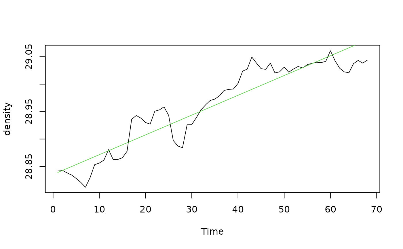
density <- ts(marphy[, "Density"])
plot(density)
Time <- time(density)

# Linear model to represent trend
density.lin <- lm(density ~ Time)
summary(density.lin)
#> 
#> Call:
#> lm(formula = density ~ Time)
#> 
#> Residuals:
#>       Min        1Q    Median        3Q       Max 
#> -0.052226 -0.018014  0.001945  0.017672  0.058895 
#> 
#> Coefficients:
#>              Estimate Std. Error t value Pr(>|t|)    
#> (Intercept) 2.884e+01  6.585e-03 4379.27   <2e-16 ***
#> Time        3.605e-03  1.659e-04   21.73   <2e-16 ***
#> ---
#> Signif. codes:  0 ‘***’ 0.001 ‘**’ 0.01 ‘*’ 0.05 ‘.’ 0.1 ‘ ’ 1
#> 
#> Residual standard error: 0.02685 on 66 degrees of freedom
#> Multiple R-squared:  0.8774,	Adjusted R-squared:  0.8755 
#> F-statistic: 472.3 on 1 and 66 DF,  p-value: < 2.2e-16
#> 
xreg <- predict(density.lin)
lines(xreg, col=3)

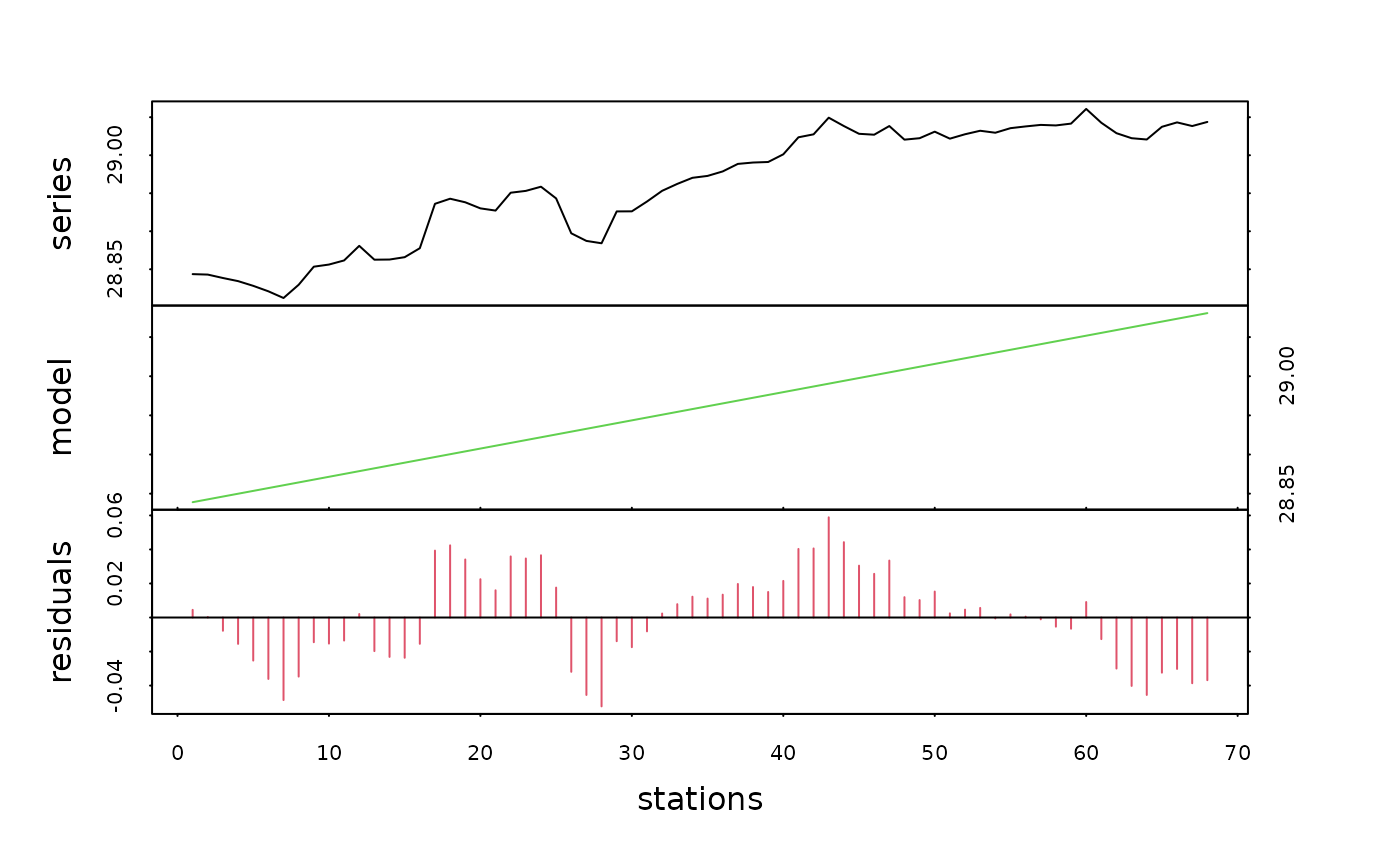
density.dec <- decreg(density, xreg)
plot(density.dec, col=c(1, 3, 2), xlab="stations")


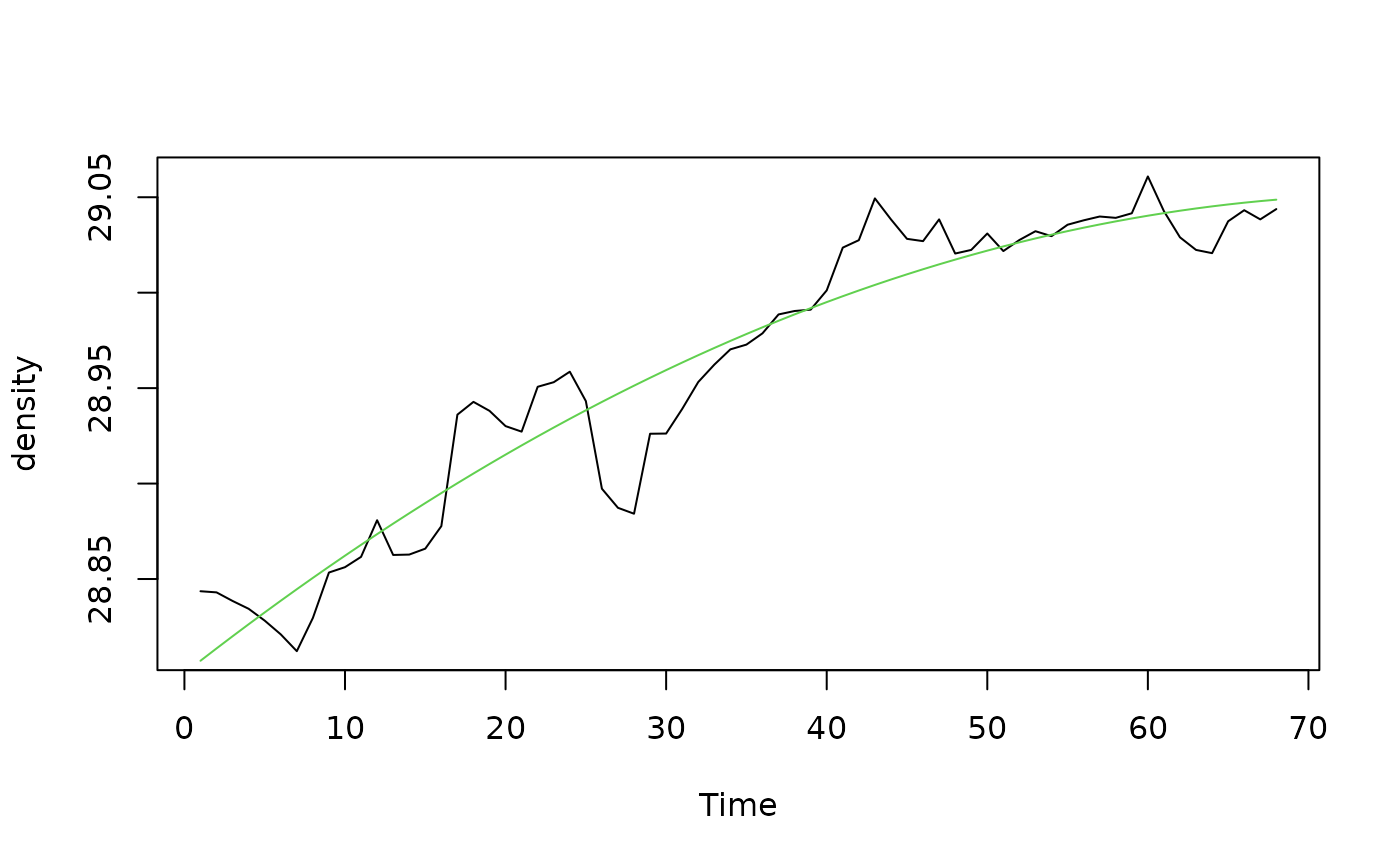
# Order 2 polynomial to represent trend
density.poly <- lm(density ~ Time + I(Time^2))
summary(density.poly)
#> 
#> Call:
#> lm(formula = density ~ Time + I(Time^2))
#> 
#> Residuals:
#>       Min        1Q    Median        3Q       Max 
#> -0.067079 -0.010665  0.001498  0.014777  0.045341 
#> 
#> Coefficients:
#>               Estimate Std. Error  t value Pr(>|t|)    
#> (Intercept)  2.880e+01  8.374e-03 3439.404  < 2e-16 ***
#> Time         6.593e-03  5.600e-04   11.773  < 2e-16 ***
#> I(Time^2)   -4.330e-05  7.866e-06   -5.505 6.73e-07 ***
#> ---
#> Signif. codes:  0 ‘***’ 0.001 ‘**’ 0.01 ‘*’ 0.05 ‘.’ 0.1 ‘ ’ 1
#> 
#> Residual standard error: 0.02234 on 65 degrees of freedom
#> Multiple R-squared:  0.9164,	Adjusted R-squared:  0.9138 
#> F-statistic: 356.2 on 2 and 65 DF,  p-value: < 2.2e-16
#> 
xreg2 <- predict(density.poly)
plot(density)
lines(xreg2, col=3)

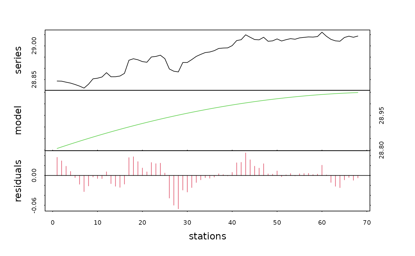
density.dec2 <- decreg(density, xreg2)
plot(density.dec2, col=c(1, 3, 2), xlab="stations")


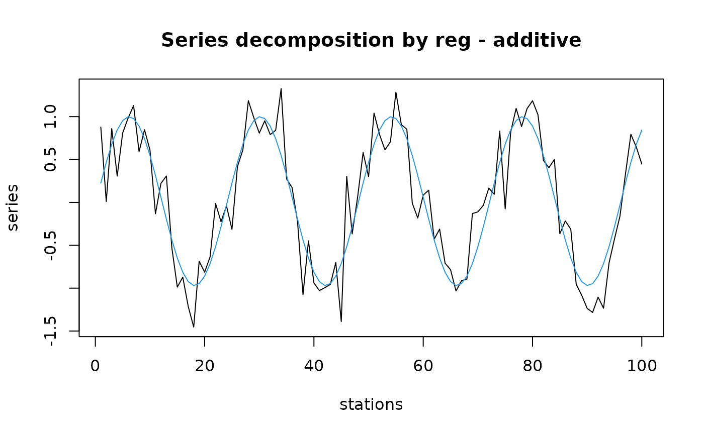
# Fit a sinusoidal model on seasonal (artificial) data
tser <- ts(sin((1:100)/12*pi)+rnorm(100, sd=0.3), start=c(1998, 4),
        frequency=24)
Time <- time(tser)
tser.sin <- lm(tser ~ I(cos(2*pi*Time)) + I(sin(2*pi*Time)))
summary(tser.sin)
#> 
#> Call:
#> lm(formula = tser ~ I(cos(2 * pi * Time)) + I(sin(2 * pi * Time)))
#> 
#> Residuals:
#>      Min       1Q   Median       3Q      Max 
#> -0.75515 -0.14794 -0.01237  0.16597  0.82122 
#> 
#> Coefficients:
#>                       Estimate Std. Error t value Pr(>|t|)    
#> (Intercept)            0.01511    0.03112   0.485    0.629    
#> I(cos(2 * pi * Time)) -0.53156    0.04450 -11.944   <2e-16 ***
#> I(sin(2 * pi * Time))  0.82928    0.04351  19.062   <2e-16 ***
#> ---
#> Signif. codes:  0 ‘***’ 0.001 ‘**’ 0.01 ‘*’ 0.05 ‘.’ 0.1 ‘ ’ 1
#> 
#> Residual standard error: 0.3108 on 97 degrees of freedom
#> Multiple R-squared:  0.8364,	Adjusted R-squared:  0.833 
#> F-statistic:   248 on 2 and 97 DF,  p-value: < 2.2e-16
#> 
tser.reg <- predict(tser.sin)
tser.dec <- decreg(tser, tser.reg)
plot(tser.dec, col=c(1, 4), xlab="stations", stack=FALSE, resid=FALSE,
        lpos=c(0, 4))

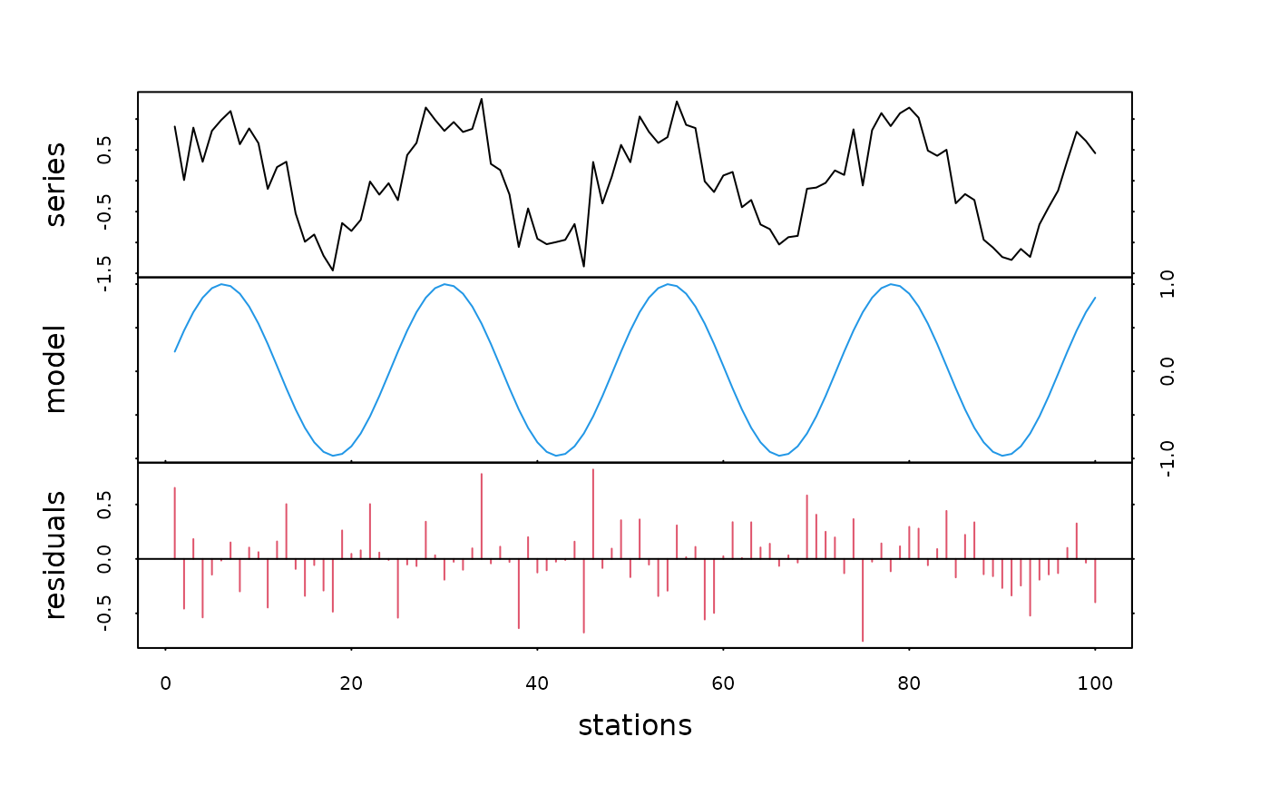
plot(tser.dec, col=c(1, 4, 2), xlab="stations")


# One can also use nonlinear models (see 'nls')
# or autoregressive models (see 'ar' and others in 'ts' library)