Adjust regulation parameters

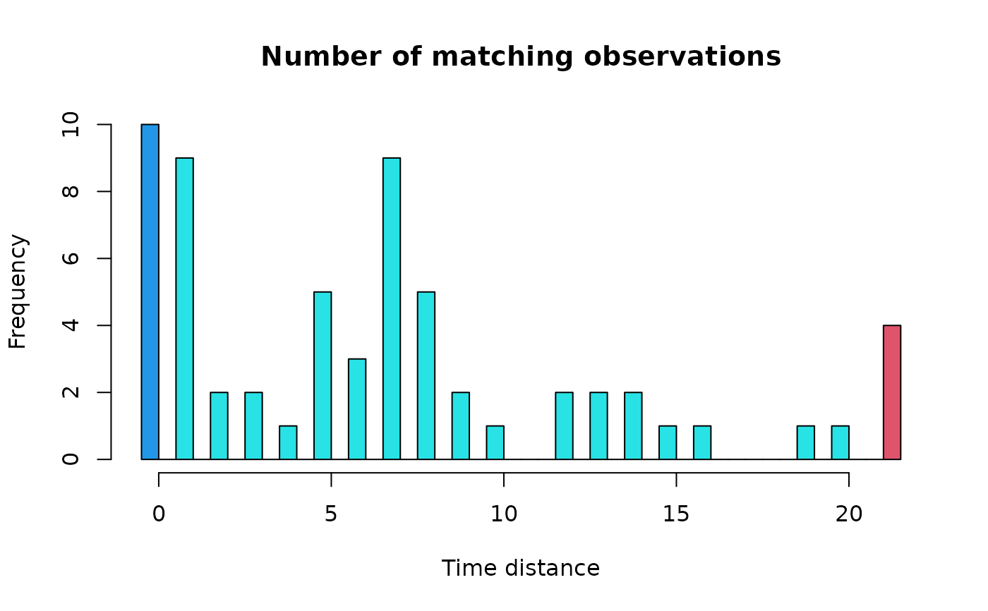
Calculate and plot an histogram of the distances between interpolated observations in a regulated time series and closest observations in the initial irregular time series. This allows to optimize the tol parameter

regul.adj(x, xmin=min(x), frequency=NULL,
     deltat=(max(x, na.rm = TRUE) - min(x, na.rm = TRUE))/(length(x) - 1),
     tol=deltat, tol.type="both", nclass=50, col=c(4, 5, 2),
     xlab=paste("Time distance"), ylab=paste("Frequency"),
     main="Number of matching observations", plotit=TRUE, ...)

Arguments

x

a vector with times corresponding to the observations in the irregular initial time series

xmin

the time corresponding to the first observation in the regular time series

frequency

the frequency of observations in the regular time series

deltat

the interval between two successive observations in the regular time series. This is the inverse of frequency. Only one of both parameters need to be given. If both are provided, frequency supersedes deltat

tol

the tolerance in the difference between two matching observations (in the original irregular series and in the regulated series). If tol=0 both values must be strictly identical; a higher value for tol allows some fuzzy matching. tol must be a round fraction of deltat and cannot be higher than it, otherwise, it is adjusted to the closest acceptable value. By default, tol=deltat

tol.type

the type of window to use for the time-tolerance: "left", "right", "both" (by default) or "none". If tol.type="left", corresponding x values are seeked in a window ]xregul-tol, xregul]. If tol.type="right", they are seeked in the window [xregul, xregul+tol[. If tol.type="both", then they are seeked in the window ]xregul-tol, xregul+tol]. If several observations are in this window, the closest one is used. Finally, if tol.type="none", then all observations in the regulated time series are interpolated (even if exactly matching observations exist!)

nclass

the number of classes to compute in the histogram. This is indicative, and will be adjusted by the algorithm to produce a nicely-formatted histogram. The default value is nclass=50. It is acceptable in many cases, but if the histogram is not correct, try a larger value

col

the three colors to use to represent respectively the fist bar (exact coincidence), the middle bars (coincidence in a certain tolerance window) and the last bar (values always interpolated). By default, col=c(4,5,2)

xlab

the label of the x-axis

ylab

the label of the y-axis

main

the main title of the graph

plotit

if plotit=TRUE then the histogram is plotted. Otherwise, it is only calculated

...

additional graph parameters for the histogram

Details

This function is complementary to regul.screen(). While the later look for the best combination of the number of observations, the interval between observations and the position of the first observation on the time-scale for the regular time series, regul.adj() look for the optimal value for tol, the tolerance window.

Value

A list with components:

params

the parameters used for the regular time-scale

match

the number of matching observations in the tolerance window

exact.match

the number of exact matching observations

match.counts

a vector with the number of matching observations for increasing values of tol

Author

Philippe Grosjean (phgrosjean@sciviews.org), Frédéric Ibanez (ibanez@obs-vlfr.fr)

See also

regul.screen, regul

Examples

# This example follows the example for regul.screen()
# where we determined that xmin=9, deltat=21, n=63, with tol=1.05
# is a good choice to regulate the irregular time series in 'releve'
data(releve)
regul.adj(releve$Day, xmin=9, deltat=21)

#> $params
#>   xmin      n deltat    tol 
#>      9     63     21     21 
#> 
#> $match
#> [1] 59
#> 
#> $exact.match
#> [1] 10
#> 
#> $match.counts
#>   0   1   2   3   4   5   6   7   8   9  10  12  13  14  15  16  19  20 Inf 
#>  10  19  21  23  24  29  32  41  46  48  49  51  53  55  56  57  58  59  63 
#> 
# The histogram indicates that it is not useful to increase tol
# more than 1.05, because few observations will be added
# except if we increase it to 5-7, but this value could be
# considered to be too large in comparison with deltat=22
# On the other hand, with tol <= 1, the number of matching
# observations will be almost divided by two!