svSweave - Sweave, Knitr and R Markdown Companion Functions

Philippe Grosjean (phgrosjean@sciviews.org)

2022-05-10

The {svSweave} package provides different functions to better manage Sweave and Knitr with LyX, a document processor that creates LaTeX code. These functions are deprecated and are not detailed here. See their help page ?clean_lyx().

The package also provides functions to automatically enumerate and reference figures, tables and equations in R Markdown documents (an alternate mechanisms to {bookdown} or {quarto} that works everywhere). Indeed, this feature is missing in the basic R Markdown documents. The various {bookdown} templates provide a \@ref(label), see bookdown cross references and Quarto simply uses @label, see quarto cross references. The functions fig(), tab() and eq() provide a different mechanism to obtain a similar result: to enumerate items and to cross-reference them in the text. Here an example of a numbered figure with its caption. In order to use these function, you must load the {svSweave} package in a (setup) chunk before you use these functions:

library(svSweave)

Numbered figures

You can use fig("my caption text") to number the caption of a figure in fig.cap=. The chunk must be named too.

hist(rnorm(50))

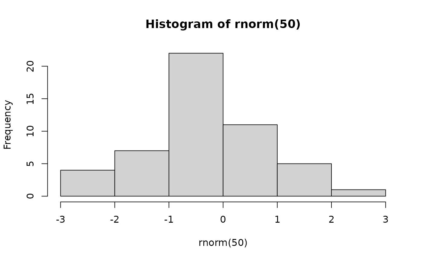
Figure 1: An example of a simple histogram.

Now, you can reference this plot in the text using fig$label (see Fig ). It also works if the first reference appears before the figure itself¹, see Fig .

boxplot(rnorm(50))

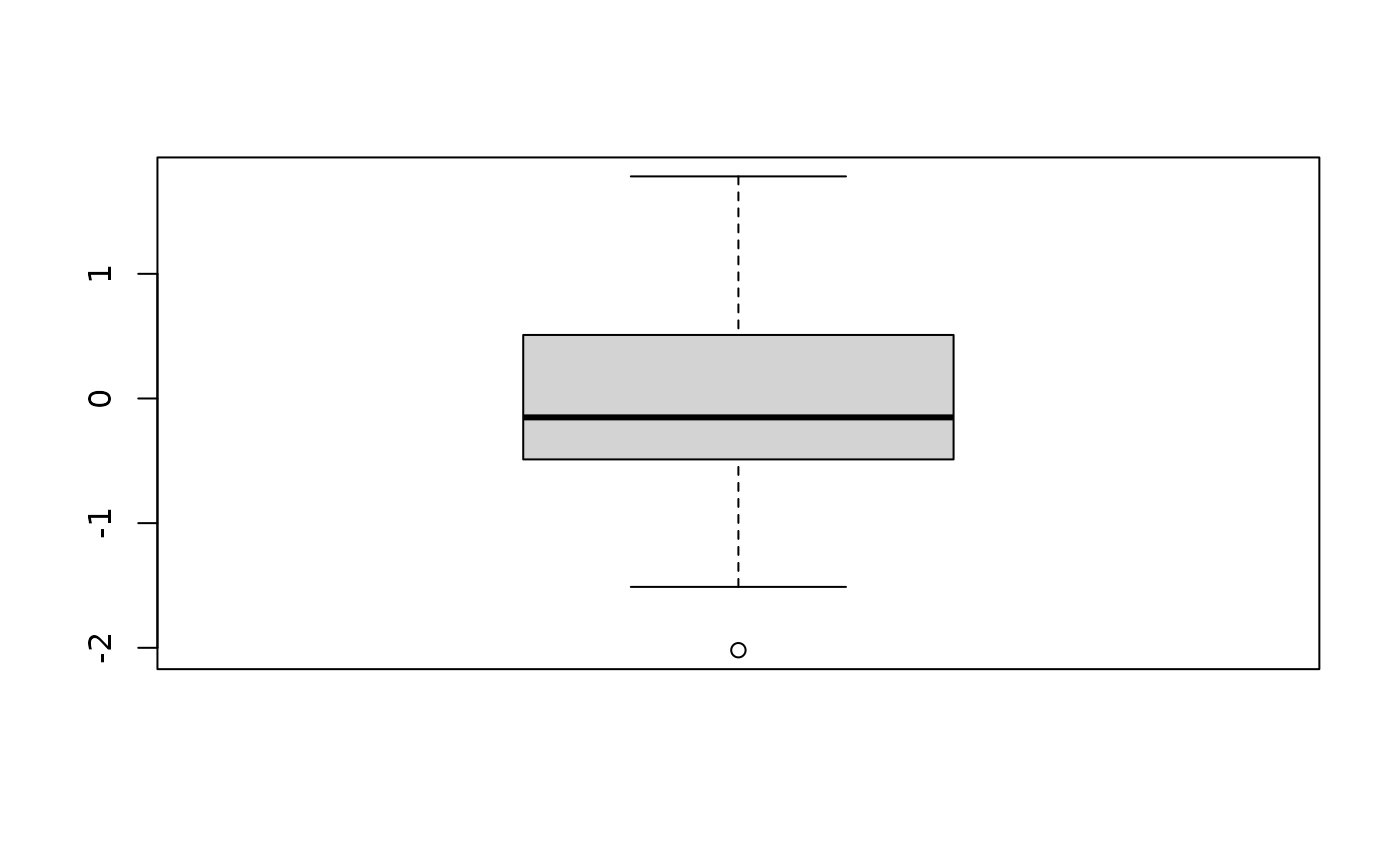
Figure 2: A second plot as an example.

Summary: produce numbered figures from labeled R chunks by indicating fig.cap = fig("...."), and reference them using fig$label in an inline R expression.

Numbered tables

The same principle works for tables using knitr::kable(). For instance, see Table .

knitr::kable(head(iris),
  caption = tab("The few first lines of the `iris` dataset."))

Table: 1: The few first lines of the iris dataset.

Sepal.Length	Sepal.Width	Petal.Length	Petal.Width	Species
5.1	3.5	1.4	0.2	setosa
4.9	3.0	1.4	0.2	setosa
4.7	3.2	1.3	0.2	setosa
4.6	3.1	1.5	0.2	setosa
5.0	3.6	1.4	0.2	setosa
5.4	3.9	1.7	0.4	setosa

A reference to cars (Table ) and to iris (Table ) again.

knitr::kable(head(cars),
  caption = tab("the first few lines of `cars`."), format = "pandoc")

Table: 2: the first few lines of cars.

speed	dist
4	2
4	10
7	4
7	22
8	16
9	10

Summary: produce numbered tables from labeled R chunks by indicating caption = tab("....") in knitr::kable(), and reference them using tab$label in an inline R expression.

Numbered equations

Finally, numbered display equations can also be constructed and cross-referenced. In the display equation, constructed with a pair of $$, you use eq(label) in an inline R expression. To reference it, you use eq$label also in an inline expression.

\[x=\frac{-b \pm \sqrt{b^2 - 4ac}}{2a} \label{eq:eqlabel} \tag{1}\]

… and I can reference Eq. \(\eqref{eq:eqlabel}\) like this.

\[\sum_{i = 0}^n{x^2} \label{eq:sum} \tag{2}\]

I can cite one Eq \(\eqref{eq:sum}\), or another one Eq \(\eqref{eq:pythagoras}\).

\[a^2+b^2=c^2 \label{eq:pythagoras} \tag{3}\]

Summary: produce numbered equations by adding eq(label) inline R expression inside a display equation, and reference to it using eq$label inside an inline R expression.

These tags work in R Markdown to compile HTML, LaTeX or Word, with some glitches remaining to eliminate for LaTeX or Word.

---

1. Take care, however, that numbering is sequential from the first call (either cross-reference, or label) in Word. You cannot cross-reference the last figure at the beginning of the document… or that last figure will be numbered “Fig. 1” there. For the other formats, it is not a problem.↩︎