

Abstract
The SciViews web site is completely refactored.
This page shows how posts are presented with the new skin.
Markdown is a simple formatting syntax for authoring HTML, PDF, and MS Word documents (among other possible formats). For more details on using R Markdown see http://rmarkdown.rstudio.com. This version supports YAML header starting and ending with three dashes (---). It also includes improvements for scientific documents (figures and tables numbering and reference, equations and equations numbering, citations and bibliographic references, …)
Here are the various R Markdown features you can use:
Headers
- Header with 6 levels, either with
#, or with underline:
Header 1
Some text…
Header 2
Some text…
Header 3
Some text…
Header 4
Some text…
Header 5
Some text…
Header 6
Some text…
An alternate syntax for headers:
Header 1
Header 2
Headers can contain formatting and links
simple link, simple code and code inside link.
Take care that a blank line is required before headers as #22 this could too easily be interpretted as a header otherwise.
- One can put identifiers after header, to allow linking to them elsewhere. Otherwise, headers are autoidentified by a special kind of reformatting of the string. Note also that references to headers can also be implicit. That is,
[linking to a header], or[linking to a header][]should work too: this is a link to the abstract.
An identified header
- One can force unnumbered titles using
{-}or{.unnumbered}(providing, of course, that the other headers are numbered).
Basic text formatting
Bold using bold or bold
Italic using italic or italic, but intra_word_underscore is not interpreted (use stars for that like in this word)
Superscript, or subscript. No space can occur inside super- or subscript. If you need it, backslash-escape the space like Pa cat.
Strikethrough with
this formatting.Formattings can be combined of course, like bold italic with superscript.
Inline code like
x <- 1, and if you need backquote inside it`@var` <- 2.Links are automatically detected like http://example.com, or can be explicitly indicated (with a different text) like some example. Note that Markdown uses also reference links. You can also put your links between angle brackets http://example.com.
You can use any UTF-8 character (at least for HTML documents (examples: µm, Ω, Æ, ∫√)…
You need to backshlash-escape punctuation you don’t want to be interpreted ad formatting code, like *foo*.
A nonbreaking space is simply an escaped space, like between “Fig.” and “3” here: Fig. 3.
A few sequences of characters produce special characters. Use of –dashes– and —em-dashes—. Three dots is ellipsis… and I can use any unicode, too, for special characters, like 😌.
Special paragraphs and other items
- Quoted text (need blank line before it to avoid misinterpretation of > inside a paragraph)
Some quoted text
With two paragraph…
More quoted
with a second paragraph within the same quote block.
And double quotation
with two paragraphs…
- Line blocks
It respect text position
Like here and you can go to the line
And a new line here
Preformatted text:
Some preformatted text using indentation
Preformatted or verbatim sections indented with four spaces of fenced (but only fenced blocks work in lists and are thus the preferred mean to do so). Fenced blocks are delimited by three or more tildes (
~) or backticks (`) and they must be separated from the surrounding using blank lines. You can use identifiers too like in this block:
Some preformatted text (like for code blocks)
using a fenced block with backticks
It is very easy to indicate a language, and syntax highlighting will be used for it:
# Idem, but with R syntax highlighting
for (i in 1:100) {
  if (i > 1) stop("Got it!")
}
It can also be specified in a more complex way, and with marks allowing to link to it:
name = raw_input('What is your name?\n')
print 'Hi, %s.' % name
Then you can link to it like here.
- Horizontal rule or page break using four or more
*,-or_optionally separated by spaces
Line breaks when ending with two or more spaces
like this paragraph. However, this is not very visible, nor usable in table. So you can also use a backslash followed by a newline
and this approach is the only way to do it in tables!You can escape special characters except in code block or inline code if you don’t want them to be interpreted as formatting marks like _here_.
Non-breaking space is entered as a backslash-escaped space (
\).Comment that do not appear in the final document are similar to HTML comments (
<!-- comment-->), but can also be entered using the[//]:syntax.
Smart punctuation is used and converts straight quotes into curly ones like ‘here’ or “here”. It will also interpret
--as en-dash –,---as em-dash —, and...as ellipses … Moreover, nonbreaking spaces are automatically used after certain items like Mr. Schmidt.Note that raw HTML (with or without interpretation of markdown inside it) can be included too.
Footnotes1 are easy to insert. Another example2. And here, I use an inline footnote3.
Text after the long note…
Lists
Unordered list (using
*,+or-)- Second level
Compact
list
of items
Loose
list
of items
Ordered list
- Second level
- Second level, second item
Back to first level
There is a mechanism to include paragraphs inside the list using indentation (don’t forget the empty line in between to start a new paragraph):
Some preformatted inside a list itemFourth item
- The fancy list extension allow for using
#.for ordered lists, as well as something like1), or(I)for instance:
- First item
- Second item
- First item
- Second item
- Third item
- Fourth item
- Definition lists are also supported (definitions must start with
:or~) and blank lines are optional between the term and its definition (loose vs compact form), but not before the term. Finally, several defintions are allowed for the same term.
- Term 1
Definition 1
- Term 2 with inline markup
Definition 2
{ some code, part of Definition 2 }Third paragraph of definition 2.
or
- Term 1
- Definition 1
- Term 2
- Definition 2a
- Definition 2b
- Numbered example lists use a sequential numbering throughout the whole document and use the
@.syntax:
- First item
- Second item
Some text
- Third item
You can give them labels (alphanumeric + character + hyphen) and refer to them later on. You can also enclose it into parentheses, but it does not change how it is displayed:
And what if I refer to it before the label like 5? Yes! It works! But unfortunately, there is no link to example 5.
- A bad example
Finally, to force ending a list, just add a comment where you want to end it (same trick applies for restarting another numbered list):
list item
another item
Formatted block with spaces does not work inside lists
third list item
Formatted block with spaces work now- New list item #1
Indent paragraphs or blocks or chunks (see hereunder) following a list item to include it in the list:
The area of a circle with a given radius is:
radius <- 3.5
pi * radius ^ 2
## [1] 38.48451As you can see, the R chunk and its associated results are included in the list element!
Images
- To insert images in your document, you use:

A nice little cat.
The official R logo.
An inline image:  . Note here that when an image appears alone in its line, it is interpreted as a figure (possibly with caption), and otherwise, it is interpeted as an inline image.
Reference links
- Reference links are done this way a linked part, or for images:
Hugo shortcodes
- Tweeter. In R Markdown, you should not use the
{{< tweet 936232450006704128 >}}syntax. Instead, you should use:
blogdown::shortcode('tweet', '936232450006704128')Excited about the new R Release? #rstats
— Lucy D’Agostino McGowan (@LucyStats) November 30, 2017
😋🎋 Welcome "Kite-Eating Tree"!
🙌🎥 gif courtesy of @pdalgd!
🤔👇 Curious about the other R release name origins? Check out our post!
🔗 https://t.co/b7XkQKwHpM pic.twitter.com/J1UNks276A
- Youtube:
- Vimeo:
- Github Gist:
- Instagram:
Figure:
Tables
There are several ways to present tables.
- Simple tables are easy to create. Header and rows must be on two lines, and column alignment is determined according to the position of the header relative to the line under it. Tables must be surrounded by empty lines and an optional caption may be added above or below the table, starting with
Table:or:(which is stripped off).
| Right | Left | Center | Default |
|---|---|---|---|
| 12 | 12 | 12 | 12 |
| 123 | 123 | 123 | 123 |
| 1 | 1 | 1 | 1 |
- The header may be omitted, but then, the ending line is mandatory.
| 12 | 12 | 12 | 12 |
| 123 | 123 | 123 | 123 |
| 1 | 1 | 1 | 1 |
- Multiline tables start and end with a line of dashes. Cells are separated by spaces (in case of a single row table, add the empty line too, otherwise, the table is interpreted as a sinlge-line table). In multiline tables, the writer tries to respect the relative size of the columns that appear in the markdown document.
| Centered Header | Default Aligned | Right Aligned | Left Aligned |
|---|---|---|---|
| First | row | 12.0 | * Example of a row that spans multiple lines. |
| Second | row | 5.0 | * Here’s another one. Note the blank line between rows. |
- Headers can be omitted too in multiline tables (note that this could be used as a simple formatting hack to place –short– material on several columns!):
| First | row | 12.0 | Example of a row that spans multiple lines. |
| Second | row | 5.0 | Here’s another one. Note the blank line between rows. |
- Grid tables (rows with
=separate headers and can be omitted for headerless tables). Apparently, more formatting is allowed in gridded tables, like list items:
| Fruit | Price | Advantages |
|---|---|---|
| Bananas | $1.34 |
|
| Oranges | $2.10 |
|
- Pipe tables look like this (beginning and end pipes are optional, and optional colon indicates alignment, header can be omitted but not the lines, and finally, although ugly, pipe do not need to align). Note that table characters like
|cannot appear in the table and this form does not support multiline tables. The semicolumn:may be used to indicate alignment inside each column, but it is an optional feature.
| Right | Left | Default | Center |
|---|---|---|---|
| 12 | 12 | 12 | 12 |
| 123 | 123 | 123 | 123 |
| * 1 | 1 | 1 | 1 |
Equations
Inline equations like \(\frac{1}{n} \sum_{i=1}^{n} x_{i} + \beta\), or \(f(\alpha, \beta) \propto x^{\alpha-1}(1-x)^{\beta-1}\).
Display equation
\[ \frac{1}{n} \sum_{i=1}^{n} x_{i} + \beta \]
Here is a more complex example spanning on several lines:
\[ \begin{aligned} \dot{x} & = \sigma(y-x) \\ \dot{y} & = \rho x - y - xz \\ \dot{z} & = -\beta z + xy \end{aligned}\]
If you feel difficult to write LaTeX equations, there are inline LateX equation editors like this one, and you don’t need to install anything on your computer to used them. Also, there is a R Studio addin provided with the bookdown R package to ease entering LaTeX equations in your R Markdown document.
Knitr chunks
The R package knitr is used to insert R code withing your Markdown document, which makes altogether an R Markdown document, usually with the .Rmd extension. Go to knitr homepage for more details.
R chunks
- A few R commands:
# This is a comment (don't use ##, since it is reserved for output!)
a <- 1 + 1 # Another comment
TRUE; NA; "Some text"
## [1] TRUE## [1] NA## [1] "Some text"summary(cars) # A table## speed dist
## Min. : 4.0 Min. : 2.00
## 1st Qu.:12.0 1st Qu.: 26.00
## Median :15.0 Median : 36.00
## Mean :15.4 Mean : 42.98
## 3rd Qu.:19.0 3rd Qu.: 56.00
## Max. :25.0 Max. :120.00- Normal output versus message versus warning versus error:
# Normal output
cat("Some text...\n")
## Some text...# A message
message("My very nice message")# Output with a warning
1:2 + 1:3## Warning in 1:2 + 1:3: longer object length is not a multiple of shorter object
## length## [1] 2 4 4# An error
non_existing_object## Error in eval(expr, envir, enclos): object 'non_existing_object' not found- R chunk with option to generate a plot5:
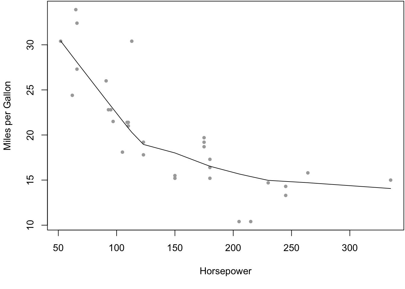
Figure 1: An example figure generated by R, from the cars dataset.
My plot is here.
- Another plot:
library(ggplot2)
qplot(speed, dist, data = cars) + geom_smooth(method = "loess")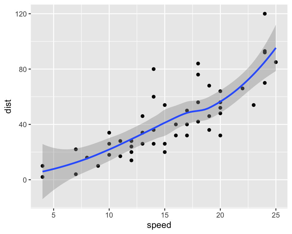
Figure 2: Distance in function of speed for the cars data set.
I can now reference this figure in the text (see this plot).
- R chunk with option to generate a table :
| Sepal.Length | Sepal.Width | Petal.Length | Petal.Width | Species |
|---|---|---|---|---|
| 5.1 | 3.5 | 1.4 | 0.2 | setosa |
| 4.9 | 3.0 | 1.4 | 0.2 | setosa |
| 4.7 | 3.2 | 1.3 | 0.2 | setosa |
| 4.6 | 3.1 | 1.5 | 0.2 | setosa |
| 5.0 | 3.6 | 1.4 | 0.2 | setosa |
| 5.4 | 3.9 | 1.7 | 0.4 | setosa |
Now, I can refer to this table (see this Table).
Tables using xtable
The xtable R package offers an alternative to output well-formatted tables in an R Markdown document:
library(xtable)
data(tli)
## Demonstrate data.frame... can also export many objects!
tli.table <- xtable(tli[1:10, ])
digits(tli.table)[c(2, 6)] <- 0
## Choose one of these!
print(tli.table, floating = FALSE, type = "html")| grade | sex | disadvg | ethnicty | tlimth | |
|---|---|---|---|---|---|
| 1 | 6 | M | YES | HISPANIC | 43 |
| 2 | 7 | M | NO | BLACK | 88 |
| 3 | 5 | F | YES | HISPANIC | 34 |
| 4 | 3 | M | YES | HISPANIC | 65 |
| 5 | 8 | M | YES | WHITE | 75 |
| 6 | 5 | M | NO | BLACK | 74 |
| 7 | 8 | F | YES | HISPANIC | 72 |
| 8 | 4 | M | YES | BLACK | 79 |
| 9 | 6 | M | NO | WHITE | 88 |
| 10 | 7 | M | YES | HISPANIC | 87 |
Tables using pander
The pander package can output various objects in pandoc:
library(pander)
# You can change default pander options:
panderOptions('table.alignment.default', function(df)
  ifelse(sapply(df, is.numeric), 'right', 'left'))
panderOptions('table.split.table', Inf)
panderOptions('big.mark', ",")
panderOptions('keep.trailing.zeros', TRUE)
pander(head(iris))| Sepal.Length | Sepal.Width | Petal.Length | Petal.Width | Species |
|---|---|---|---|---|
| 5.1 | 3.5 | 1.4 | 0.2 | setosa |
| 4.9 | 3.0 | 1.4 | 0.2 | setosa |
| 4.7 | 3.2 | 1.3 | 0.2 | setosa |
| 4.6 | 3.1 | 1.5 | 0.2 | setosa |
| 5.0 | 3.6 | 1.4 | 0.2 | setosa |
| 5.4 | 3.9 | 1.7 | 0.4 | setosa |
Tables using flextable
The flextable package allows for fine customization of the formatted table:
library(flextable)library(dplyr)library(flow)
mtcars %>.%
group_by(., cyl, am) %>.%
summarise(., avg = mean(mpg)) %>.%
flextable(.) %>.%
bg(., bg = '#c7deff', part = 'header')cyl | am | avg |
4 | 0 | 22.90000 |
4 | 1 | 28.07500 |
6 | 0 | 19.12500 |
6 | 1 | 20.56667 |
8 | 0 | 15.05000 |
8 | 1 | 15.40000 |
There are many other packages to output well-formatted tables from R objects, like: stargazer, table1, tables, formattable, htmlTable, huxtable, kableExtra, pixiedust, tangram, texreg, ztable, etc.
Inline R expressions and special chunks
Inline R expression like 2, or R version 3.6.3 (2020-02-29).
Rcpp code chunks can also be included in your document:
#include <Rcpp.h>

// [[Rcpp::export]]
int fibonacci(const int x) {
    if (x == 0 || x == 1) return(x);
    return (fibonacci(x - 1)) + fibonacci(x - 2);
}
Because fibonacci was defined with the Rcpp::export attribute it can now be called as a normal R function:
fibonacci(10L)## [1] 55fibonacci(20L)## [1] 6765- An R chunk that is displayed, but not executed:
library(knitr)
knit('R Markdown V2 Syntax.Rmd')- A Python chunk:
import sys
print(sys.version)
## 2.7.16 (default, Apr 17 2020, 18:29:03)
## [GCC 4.2.1 Compatible Apple LLVM 11.0.3 (clang-1103.0.29.20) (-macos10.15-objc-Icons
You have both the font awesome, and the themify icons. You need to create an object of class “fa fa-xxxx”, or “ti-xxxx”, where “xxxx” is an icon in the collection. Here is an example from font awesome , and here is one from themify: . You can use these icons everywhere!
Citations
Thanks to Pandoc, it is rather easy to insert citations in your text. First, you need to specify a bibliography file in a YAML section. A number of formats are supported, but to remain compatible with LaTeX, use BibTeX (.bibtex) or BibLaTeX (.bib) format only. Note that the bibliography folder, like for figures is two folders ahead in the relative path, i.e., ../../bibliography/<my-file.bib>.
The file we use here is named bibliography.bib. It is enough to refer to it in a YAML section. However, we will also add more reference to the bibliography later on. So, we first copy this file into bibliography-full.bib and then, we refer to the later file instead.
- A
referencesfield can also be included in a YAML section for self-contained bibliography (and you can use both at the same time!).
- The R package
knitcitationsuses pandoc citations, but enhances its mechanisms by allowing to add citations by DOIs or URL and by linking to cited papers directly. You need to start loading the package and clean up citations.
You can use references citations contained in your bibliography inside square brackets, separated by semicolons and each citation must be composed using @ + citation identifier. For instance (Greenwade 1993; Fenner 2012), or (see Fenner 2012, pp. 12–17; also Greenwade 1993, ch. 2). Use a minus sign before the reference to suppress mention of the author: as Greenwade (1993) indicated, “bla bla”. You can also write the inline citation this way: Fenner (2012, p. 10) says “bla”.
Finally, you can include citations in the references without citing them by using a nocite entry in a YAML block:
---
nocite:
 | @item1, @item2
---
By default, the Chicago author-date format is used by Pandoc, but you can use a different style by specifying a CSL 1.0 style in a csl metadata entry in a YAML block. The RStudio rmarkdown site indicates two interesting pages to get CSL files: CSL official repository and Zotero styles page that allows easy browsing. Here, we use the Marine Biology style.
As already mentioned, an addition to this mechanism is provided by the knitcitations package that allows to build citations from DOIs, or URL into Pandoc-compatible citations. The question of independent .bib file, and/or need for an Internet link to compile the document is discussed here http://blog.martinfenner.org/2013/06/19/citations-in-scholarly-markdown/.
One big lack in this approach is no link between the citation and the reference.
Now for knitcitations citations… We can add a citation by DOI (Abrams et al. 2012), or Boettiger and Hastings (2013). Since a citation like name_year is automatically created, one do not need to recite the same items by DOI, but one can cite like this (Abrams et al. 2012), which should be the same as (Abrams et al. 2012). Finally, one can also cite R bibentry objects directly, like (Xie 2014, 2015, 2020). All these approaches are combinable with traditional pandoc citations, providing these citations are already included in the .bib file.
Finally, don’t forget to generate the complete .bib file by appending the following last R chunk into your document in order to add the knitcitations in your document properly:
write.bibtex(file = "../../bibliography/bibliography-full.bib", append = TRUE)Note how the references are included automatically at the end of the document. Do not forget to put an adequate header by yourself!
References
Abrams PA, Ruokolainen L, Shuter BJ, McCann KS (2012) Harvesting creates ecological traps: Consequences of invisible mortality risks in predatorprey metacommunities. Ecology 93:281–293. https://doi.org/10.1890/11-0011.1
Boettiger C, Hastings A (2013) No early warning signals for stochastic transitions: Insights from large deviation theory. Proceedings of the Royal Society B: Biological Sciences 280:20131372. https://doi.org/10.1098/rspb.2013.1372
Fenner M (2012) One-click science marketing. Nature Materials 11:261–263. https://doi.org/10.1038/nmat3283
Greenwade G (1993) The Comprehensive Tex Archive Network (CTAN). TUGBoat 14:342–351
Xie Y (2020) Knitr: A general-purpose package for dynamic report generation in r
Xie Y (2015) Dynamic documents with R and knitr, 2nd edn. Chapman; Hall/CRC, Boca Raton, Florida
Xie Y (2014) Knitr: A comprehensive tool for reproducible research in R. In: Stodden V, Leisch F, Peng RD (eds) Implementing reproducible computational research. Chapman; Hall/CRC
This is my simple footnote.↩︎
Footnotes can span on multiple paragraphs, providing you indent them with four spaces:
- A list item
Another paragraph belonging to the note.↩︎
Inline footnotes are easier to write right in your text, but they can only span on a single paragraph.↩︎
Note that you cannot include the number inside the link, unfortunately.↩︎
Do not use underscore
_in the label of your chunk to use it as a link!↩︎
