Compute and plot a semi-variogram

Compute a classical semi-variogram for a single regular time series

vario(x, max.dist=length(x)/3, plotit=TRUE, vario.data=NULL)

Arguments

x: a vector or an univariate time series
max.dist: the maximum distance to calculate. By default, it is the third of the number of observations
plotit: If plotit=TRUE then the graph of the semi-variogram is plotted
vario.data: data coming from a previous call to vario(). Call the function again with these data to plot the corresponding graph

Value

A data frame containing distance and semi-variogram values

References

David, M., 1977. Developments in geomathematics. Tome 2: Geostatistical or reserve estimation. Elsevier Scientific, Amsterdam. 364 pp.

Delhomme, J.P., 1978. Applications de la théorie des variables régionalisées dans les sciences de l'eau. Bull. BRGM, section 3 n°4:341-375.

Matheron, G., 1971. La théorie des variables régionalisées et ses applications. Cahiers du Centre de Morphologie Mathématique de Fontainebleau. Fasc. 5 ENSMP, Paris. 212 pp.

Author

Frédéric Ibanez (ibanez@obs-vlfr.fr), Philippe Grosjean (phgrosjean@sciviews.org)

Examples

data(bnr)
vario(bnr[, 4])

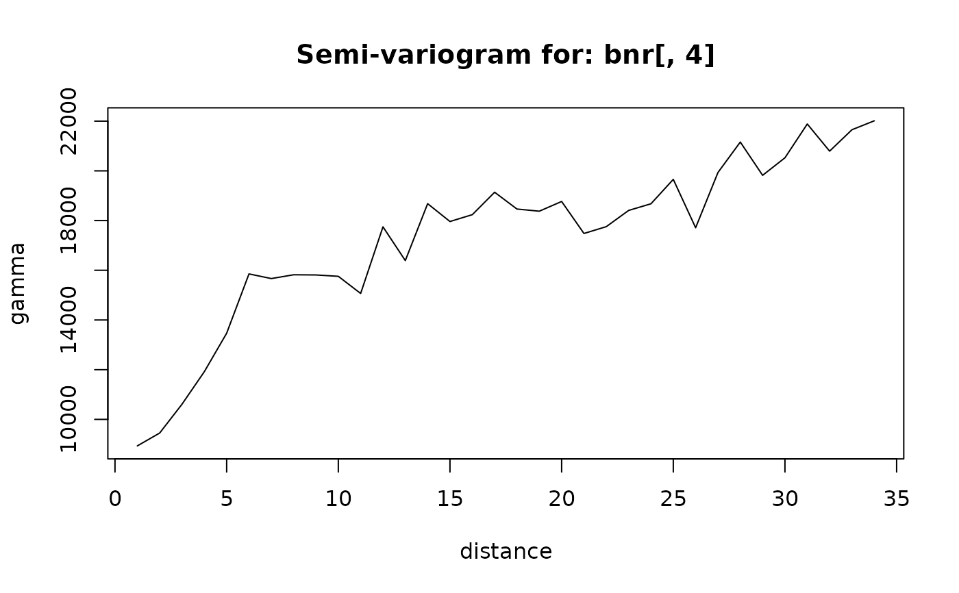#>    distance semivario
#> 1         1  8933.284
#> 2         2  9450.129
#> 3         3 10609.430
#> 4         4 11919.288
#> 5         5 13466.546
#> 6         6 15853.098
#> 7         7 15666.052
#> 8         8 15818.568
#> 9         9 15811.266
#> 10       10 15756.645
#> 11       11 15066.837
#> 12       12 17747.786
#> 13       13 16389.750
#> 14       14 18679.669
#> 15       15 17961.426
#> 16       16 18236.943
#> 17       17 19139.413
#> 18       18 18463.482
#> 19       19 18376.732
#> 20       20 18767.747
#> 21       21 17480.317
#> 22       22 17754.858
#> 23       23 18407.075
#> 24       24 18675.184
#> 25       25 19656.635
#> 26       26 17710.909
#> 27       27 19933.375
#> 28       28 21158.673
#> 29       29 19820.446
#> 30       30 20525.432
#> 31       31 21885.569
#> 32       32 20792.761
#> 33       33 21654.493
#> 34       34 22013.464